Instructor’s Manual and Testbank
To accompany
Basic Environmental Technology:
Water Supply, Waste Management and Pollution Control
6th Edition
Jerry A. Nathanson, PE
Richard A. Schneider
Upper Saddle River, New Jersey
Columbus, Ohio
,__________________________________________________________________________________
Copyright © 2015, 2008, 2003, 2000, 1997 by Pearson Education, Inc., Upper Saddle River,
New Jersey 07458.
Pearson Prentice Hall. All rights reserved. Printed in the United States of America. This publication
is protected by Copyright and permission should be obtained from the publisher prior to any
prohibited reproduction, storage in a retrieval system, or transmission in any form or by any means,
electronic, mechanical, photocopying, recording, or likewise. For information regarding
permission(s), write to: Rights and Permissions Department.
Pearson Prentice Hall™ is a trademark of Pearson Education, Inc.
Pearson® is a registered trademark of Pearson plc
Prentice Hall® is a registered trademark of Pearson Education, Inc.
Instructors of classes using Nathanson and Schneider, Basic Environmental Technology: Water
Supply, Waste Management and Pollution Control, Sixth Edition may reproduce material from the
instructor’s manual for classroom use.
10 9 8 7 6 5 4 3 2 1
ISBN-13: 978-0-13-284048-4
ISBN-10: 0-13-284048-0
, Table of Contents
Chapter 1 1
Chapter 2 2
Chapter 3 5
Chapter 4 8
Chapter 5 10
Chapter 6 12
Chapter 7 14
Chapter 8 18
Chapter 9 20
Chapter 10 23
Chapter 11 26
Chapter 12 29
Chapter 13 29
Chapter 14 32
Supplemental Problems 35
Multiple Choice and True/False 36
Answers to Multiple Choice and True/False 50
Supplemental Problems 52
, 1
Basic Environmental Technology - Solutions Manual Sixth Edition
This manual provides instructors with (a) text page references where answers to the end-of-chapter
Review Questions can be found and worked-out solutions to each of the Practice Problems.
Additional materials including supplemental problems and projects.
Generally, answers to end-of-chapter Practice Problems are rounded-off to reflect the precision of
the data and/or the accuracy of the assumed factors in the problems. These answers are also listed
in Appendix G of the text for students to use in checking their work. (The authors have made every
attempt to keep errors to a minimum. They can be notified of any mistakes that may be found in the
text or in this manual at: or )
CHAPTER 1 - BASIC CONCEPTS
Review Question Page References
(1) 1 (17) 15
(2) 2, 3 (18) 15
(3) 6 (19) 16
(4) 6 (20) 16, 17
(5) 6 (21) 17
(6) 7 (22) 17
(7) 8 (23) 18
(8) 9 (24) 19
(9) 9, 10 (25) 19
(10) 9, 10 (26) 20
(11) 10 (27) 20
(12) 10 (28) 20
(13) 11 (29) 13
(14) 12 (30) 14
(15) 12, 13 (31) 20, 21
(16) 12
(There are no Practice Problems for Chapter 1)
, 2
CHAPTER 2 - HYDRAULICS
Review Question Page References
(1) 24 (8) 30 (15) 42
(2) 24 (9) 31 (16) 44
(3) 25 (10) 32 (17) 44
(4) 25 (11) 33 (18) 44
(5) 27 (12) 35 (19) 45
(6) 28 (13) 36 (20) 45
(7) 30 (14) 40-42 (21) 46
(22) www.iihr.uiowa.edu/research
Solutions to Practice Problems
1. P = 0.43 x h (Equation 2-2b)
P = 0.43 x 50 ft = 22 psi at the bottom of the reservoir
P = 0.43 x (50 -30) = 0.43 x 20 ft = 8.6 psi above the bottom
2. h = 0.1 x P = 0.1 x 50 = 5 m (Equation 2-3a)
3. Depth of water above the valve: h = (78 m -50 m) + 2 m = 30 m
P = 9.8 x h = 9.8 x 30 = 294 kPa ≈ 290 kPa (Equation 2-2a)
4. h = 2.3 x P = 2.3 x 50 = 115 ft, in the water main
h = 115 - 40 = 75 ft
P = 0.43 x 75 = 32 psi, 40 ft above the main (Equation 2-2b)
5. Gage pressure P = 30 + 9.8 x 1 = 39.8 kPa ≈ 40 kPa
Pressure head (in tube) = 0.1 x 40 kPa = 4 m
6. Q= A x V (Eq. 2-4), therefore V = Q/A
A = πD2/4 = π (0.3)2/4 = 0.0707 m2
100L/s x 1 m3/1000L=0.1 m3/s
V = 0.1 m3/s 0.707m2 = 1.4 m/s
7. Q = (500 gal/min) x (1 min/60 sec) x (1 ft3/7.5 gal) = 1.11 cfs
A = Q/V (from Eq. 2-4)
A = 1.11 ft3/sec /1.4 ft/sec = 0.794 ft2
A = πD2/4, therefore D = √4A/π = √(4)(0.794)/π = 1 ft = 12 in.
8. Q=A1 x V1 = A2 x V2 (Eq.2-5)
Since A = πD2/4, we can write
D12 xV1 = D22 xV2 and V2 =V1 x (D12 /D22)
In the constriction, V2 = (2 m/s) x (4) = 8 m/s
, 3
9. Area of pipe A = π(0.3)2/4 = 0.0707 m2
Area of pipe B = π(0.1)2/4 = 0.00785 m2
Area of pipe C= π(0.2)2/4 = 0.03142 m2
QA = QB +QC = 0.00785 m2 x 2 m/s + 0.03142 m2 x 1 m/s
= 0.04712 m3/s (from continuity of flow: QIN = QOUT)
VA = QA/AA = 0.4712/0.0707 ≈ 0.67 m/s (from Eq. 2-4)
10. p1/w + V12/2g = p2/W + V22/2g (Eq.2-8)
A1 = π(1.33)2/4 = 1.4 ft2 A2 = π(0.67)2/4 = 0.349 ft2
V1 = 6/1.4 = 4.29 ft/sec V2 = 6/0.349 = 17.2 ft/sec
w = 62.4 Ib/ft3 and g = 32.2 ft/sec2
From Eq. 2-8, and multiplying psi x 144 in2/ft2 to get Ib/ft2
50(144)/62.4 + 4.292/2(32.2) = p2(144)/62.4 + 17.22/2(32.2)
115.38 + 0.28578 = 2.3076p2 + 4.5937
p2 = 111.07 /2.307 ≈ 48 psi
11. p1/w + v12/2g = p2/w + v22/2g (Eq.2-8)
A1 = π(0.300) / 4 = 0.0707 m A2 = π(0.1 00)2/4 = 0.00785 m2
2 2
Q= 50 L/s x 1 m3/1000 L = 0.05 m3/s
V1 = 0.05/0.0707 = 0.70721 m/sec V2 = 0.05/0.00785 = 6.369 m/sec
w = 9.81 kN/m3 and g = 9.81 m/s2; From Eq. 2-8,
700/2(9.81) + 0.707212/2(9.81) = p2/2(9.81) + 6.3692/2(9.81)
35.67789 + 0.02549 = 0.05097p2 + 2.06775 and p2 = 660 kPa
12. From Figure 2.15, with Q = 200 L/s and D = 600 mm, read S = 0.0013. Therefore hL= S x L =
0.0013 x 1000 m = 1.3 m
Pressure drop p = 9.8 x 1.3 ≈ 12.7 ≈ 13 kPa per km
13. hL= 2.3 x 20 = 46 ft and S = 46/5280 = 0.0087 (where 1 mi = 5280 ft)
From Figure 2.15, with Q = 1000 gpm and S = 0.0087, read D = 10.3 in.
Use a 12 in. standard diameter pipe
14. S = 10/1000 = 0.01
From the nomograph (Figure 2.15) read Q ≈ 100 L/s = 0.1 m3/s
Check with Eq. 2-9: Q = 0.28 x 100 x 0.32.63 x 0.010.54 ≈ 0.1 m3/s OK
15. Use (Eq. 2-10): Q = C x A2 x {(2g(p1 –p2)/w)/(1 -(A2/A1)2}1/2
where A1 = π(6)2/4 = 28.27 in2 and A2 = π(3)2/4 = 7.07 in2
g = 32.2 ft/s2 = 386.4 in/s2
w = 62.4 Ib/ft3 x 1 ft3/123 in3 = 0.0361 Ib/in3
Q = 0.98 x 7.07 x {(2(386.4)(10)/0.0361 )1(1 -(7.07/28.27)2)} 1/2
, 4
Q= 0.98 x 7.07 x √228,354 = 3311 in3/s = 1.9 cfs ≈ 2 cfs
16. Use (Eq. 2-10): Q = C x A2 x {(2g(p1 – p2)/w)/(1 -(A2/ A1 )2)} 1/2
A1= π(0.15)2/4 = 0.01767 m2 and A2 = π(0.075)2/4 = 0.00442 m2
g = 9.81 m/s2 w = 9.81 kN/m3
1 -(A2/ A1 )2 = 1 -(0.00442/0.01767)2 = 0.93743
Q = 0.98 x 0.00442 x {(2(9.81)(100)/9.81)/0.93743)} 1/2 = 0.063 m3/s
(or, Q = 0.063 m3/s x 1000 L/m3 = 63 L/s)
17. Use Manning's nomograph (Figure 2.21): With D = 800 mm = 80 cm, n=0.013 and S = 0.2% =
0.002, read Q= 0.56 m3/s = 560 L/s and V = 1.17 m/s
18. S = 1.5/1000 = 0.015; from Fig. 2.21, Q ≈ 1800 gpm and V ≈ 2.3 ft/s
19. Q= 200 L/s = 0.2 m3/s; from Fig. 2.21, D ≈ 42 cm; Use 450 mm pipe
20. Q = 7 mgd = 7,000,000 gal/day x 1 day/1440 min ≈ 4900 gpm
From Fig. 2.21, with n=0.013, D=36 in and Q=4900 gpm: S = 0.00027, V = 1.54 ft/s Since 1.54
ft/s is less than the minimum self-cleansing velocity of
2 ft/s, it is necessary to increase the slope of the 36 in pipe.
From Fig. 2.21, with 36 in and 2 ft/s: S = 0.00047 = 0.047% = 0.05%
21. For full-flow conditions, with D = 300 mm and S = 0.02, read from
Fig. 2.21: Q = 0.135 m3/s = 135 L/s and V = 2m/s
q/Q = 50/135 = 0.37 From Fig. 2.22, d/D = 0.42 and v/V = 0.92
Depth at partial flow d = 0.42 x 300 = 126 mm ≈ 130 mm
Velocity at partial flow v = 0.92 x 2 ≈ 1.8 m/s
22. For full-flow conditions, from Fig. 2.21 read Q = 1800 gpm. From Fig. 2.22, the maximum value
of q/Q = 1.08 when d/D = 0.93. Therefore, the highest discharge capacity for the 18" in pipe,
qmax = 1800 x 1.08 ≈ 1900 gpm,
would occur at a depth of d = 18 x 0.93 ≈ 17 in.
23. For full-flow conditions, from Fig. 2.21 read Q = 0.55 m3/s = 550 L/s. From Fig.2.22, the
maximum value of v/V = 1.15 when d/D = 0.82. Therefore, the highest flow velocity for the
900 mm pipe, vmax = 0.9 x 1.15 ≈ 1 m/s, would occur at a depth of d = 900 x 0.82 ≈ 740 mm.
When the flow occurs at that depth, q/Q = 1.05 and the discharge q = 580 L/s
24. S = 0.5/100 = 0.005
For full-flow conditions, Q = 0.44 m3/s = 440 L/s and V = 1.6 m/s
Since d/D = 200/600 = 0.33, from Fig. 2.22 q/Q = 0.23 and v/V = 0.8 Therefore, q = 440 x
0.23 ≈ 100 L/s and v = 1.6 x 0.8 ≈ 1.3 m/s
25. Q = A x V = 2 x 0.75 x 25/75 = 0.5 m3/s = 500 L/s
, 5
26. From Eq. 2-12, Q = 2.5 x (4/12)2.5 = 0.16 cfs
27. 150 mm x 1 in/25.4 mm x 1 ft/12 in = 0.492 ft
From Eq. 2-12, Q = 2.5 x (0.492)2.5 = 0.425 cfs x 28.32 L/ft3 ≈ 12 L/s
28. From Eq. 2-13, Q = 3.4 x (20/12) x (10/12)1.5 = 4.3 cfs ≈ 120 L/s
CHAPTER 3 - HYDROLOGY
Review Question Page References
(1) 50 (13) 56 (25) 69
(2) 50 (14) 58 (26) 69
(3) 50 (15) 59 (27) 69
(4) 51 (16) 59 (28) 70
(5) 52 (17) 62 (29) 70
(6) 52,53 (18) 62 (30) 71
(7) 54 (19) 62,63
(8) 54 (20) 63
(9) 55 (21) 64
(10) 55 (22) 66
(11) 55 (23) 67
(12) 55 (24) 69
Solutions to Practice Problems
1. Intensity = 500 mm/ 10 h = 50 mm/h
Volume = depth x area = 0.5 m x 750 000 m2 = 375 000 m2 = 375 ML
2. Intensity = 1 in./0.5.h = 2 in./h
Volume = depth x area = 1 in. x 1 ft/12 in. x 96 ac = 8 ac-ft
Volume = 8 ac-ft x 43,560 ft2/ac ≈ 350,000 ft3
3. (a) 100 mm/h (4 in./h); (b) 45 mm/h (1.7 in./h); (c) 50 mm/h (2 in./h)
4. 75 mm/0.5 h = 150 mm/h; line up 30 min and 150 mm/h in Fig. 3.5. The intersection falls on the
100-yr storm curve. The probability of a greater storm occurring within the next year is P =
1/100 = 0.01 = 1 %
5. From Eq. 3-3, i = 3000/(90 + 20) = 27 mm/h
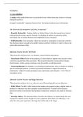
6. P = Low Flow Rank Probability Low Flow Rank Probability 1/N = 1/20 = 0.05 = 5%
57 1 0.059 45 9 0.529
7. 53 2 0.117 44 10 0.588
50 3 0.176 42 11 0.617
50 4 0.235 11 12 0.706
50 5 0.294 40 13 0.765
48 6 0.353 39 14 0.824
47 7 0.412 36 15 0.882
45 8 0.471 33 16 0.941
, 6
Multiply vertical axis values on Figure 3.16 by 10, and plot Low Flow versus Probability. Read
MA7CD10 flow to be approximately 35m3/s (where the recurrence value = 10 yrs.)
8. a and b
, 7
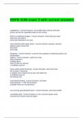
9.
10. V = K x S (Darcy's Law, Equation 3-4)
V = 0.05 mm/s x 0.5/100 = 0.05 x 0.005 = 0.00025 mm/s
V = 0.00025 mm/s x 3600 s/h x 24 h/d = 0.9 mm/h ≈ 22 mm/d
11. K = VIS (From.Eq.3-4)
V = 0.05 m/h x 1000mm/m x 1h/3600 s = 0.0139 mm/s
K = 0.0139/0.035 ≈ 0.4 mm/s (For sand, K = 0.01 to 10 mm/s)
12. Yield = 2 m3/h/m x 15 m = 30 m3/h
10% of 30 = 3; new yield ≈ 33 m3/h
To accompany
Basic Environmental Technology:
Water Supply, Waste Management and Pollution Control
6th Edition
Jerry A. Nathanson, PE
Richard A. Schneider
Upper Saddle River, New Jersey
Columbus, Ohio
,__________________________________________________________________________________
Copyright © 2015, 2008, 2003, 2000, 1997 by Pearson Education, Inc., Upper Saddle River,
New Jersey 07458.
Pearson Prentice Hall. All rights reserved. Printed in the United States of America. This publication
is protected by Copyright and permission should be obtained from the publisher prior to any
prohibited reproduction, storage in a retrieval system, or transmission in any form or by any means,
electronic, mechanical, photocopying, recording, or likewise. For information regarding
permission(s), write to: Rights and Permissions Department.
Pearson Prentice Hall™ is a trademark of Pearson Education, Inc.
Pearson® is a registered trademark of Pearson plc
Prentice Hall® is a registered trademark of Pearson Education, Inc.
Instructors of classes using Nathanson and Schneider, Basic Environmental Technology: Water
Supply, Waste Management and Pollution Control, Sixth Edition may reproduce material from the
instructor’s manual for classroom use.
10 9 8 7 6 5 4 3 2 1
ISBN-13: 978-0-13-284048-4
ISBN-10: 0-13-284048-0
, Table of Contents
Chapter 1 1
Chapter 2 2
Chapter 3 5
Chapter 4 8
Chapter 5 10
Chapter 6 12
Chapter 7 14
Chapter 8 18
Chapter 9 20
Chapter 10 23
Chapter 11 26
Chapter 12 29
Chapter 13 29
Chapter 14 32
Supplemental Problems 35
Multiple Choice and True/False 36
Answers to Multiple Choice and True/False 50
Supplemental Problems 52
, 1
Basic Environmental Technology - Solutions Manual Sixth Edition
This manual provides instructors with (a) text page references where answers to the end-of-chapter
Review Questions can be found and worked-out solutions to each of the Practice Problems.
Additional materials including supplemental problems and projects.
Generally, answers to end-of-chapter Practice Problems are rounded-off to reflect the precision of
the data and/or the accuracy of the assumed factors in the problems. These answers are also listed
in Appendix G of the text for students to use in checking their work. (The authors have made every
attempt to keep errors to a minimum. They can be notified of any mistakes that may be found in the
text or in this manual at: or )
CHAPTER 1 - BASIC CONCEPTS
Review Question Page References
(1) 1 (17) 15
(2) 2, 3 (18) 15
(3) 6 (19) 16
(4) 6 (20) 16, 17
(5) 6 (21) 17
(6) 7 (22) 17
(7) 8 (23) 18
(8) 9 (24) 19
(9) 9, 10 (25) 19
(10) 9, 10 (26) 20
(11) 10 (27) 20
(12) 10 (28) 20
(13) 11 (29) 13
(14) 12 (30) 14
(15) 12, 13 (31) 20, 21
(16) 12
(There are no Practice Problems for Chapter 1)
, 2
CHAPTER 2 - HYDRAULICS
Review Question Page References
(1) 24 (8) 30 (15) 42
(2) 24 (9) 31 (16) 44
(3) 25 (10) 32 (17) 44
(4) 25 (11) 33 (18) 44
(5) 27 (12) 35 (19) 45
(6) 28 (13) 36 (20) 45
(7) 30 (14) 40-42 (21) 46
(22) www.iihr.uiowa.edu/research
Solutions to Practice Problems
1. P = 0.43 x h (Equation 2-2b)
P = 0.43 x 50 ft = 22 psi at the bottom of the reservoir
P = 0.43 x (50 -30) = 0.43 x 20 ft = 8.6 psi above the bottom
2. h = 0.1 x P = 0.1 x 50 = 5 m (Equation 2-3a)
3. Depth of water above the valve: h = (78 m -50 m) + 2 m = 30 m
P = 9.8 x h = 9.8 x 30 = 294 kPa ≈ 290 kPa (Equation 2-2a)
4. h = 2.3 x P = 2.3 x 50 = 115 ft, in the water main
h = 115 - 40 = 75 ft
P = 0.43 x 75 = 32 psi, 40 ft above the main (Equation 2-2b)
5. Gage pressure P = 30 + 9.8 x 1 = 39.8 kPa ≈ 40 kPa
Pressure head (in tube) = 0.1 x 40 kPa = 4 m
6. Q= A x V (Eq. 2-4), therefore V = Q/A
A = πD2/4 = π (0.3)2/4 = 0.0707 m2
100L/s x 1 m3/1000L=0.1 m3/s
V = 0.1 m3/s 0.707m2 = 1.4 m/s
7. Q = (500 gal/min) x (1 min/60 sec) x (1 ft3/7.5 gal) = 1.11 cfs
A = Q/V (from Eq. 2-4)
A = 1.11 ft3/sec /1.4 ft/sec = 0.794 ft2
A = πD2/4, therefore D = √4A/π = √(4)(0.794)/π = 1 ft = 12 in.
8. Q=A1 x V1 = A2 x V2 (Eq.2-5)
Since A = πD2/4, we can write
D12 xV1 = D22 xV2 and V2 =V1 x (D12 /D22)
In the constriction, V2 = (2 m/s) x (4) = 8 m/s
, 3
9. Area of pipe A = π(0.3)2/4 = 0.0707 m2
Area of pipe B = π(0.1)2/4 = 0.00785 m2
Area of pipe C= π(0.2)2/4 = 0.03142 m2
QA = QB +QC = 0.00785 m2 x 2 m/s + 0.03142 m2 x 1 m/s
= 0.04712 m3/s (from continuity of flow: QIN = QOUT)
VA = QA/AA = 0.4712/0.0707 ≈ 0.67 m/s (from Eq. 2-4)
10. p1/w + V12/2g = p2/W + V22/2g (Eq.2-8)
A1 = π(1.33)2/4 = 1.4 ft2 A2 = π(0.67)2/4 = 0.349 ft2
V1 = 6/1.4 = 4.29 ft/sec V2 = 6/0.349 = 17.2 ft/sec
w = 62.4 Ib/ft3 and g = 32.2 ft/sec2
From Eq. 2-8, and multiplying psi x 144 in2/ft2 to get Ib/ft2
50(144)/62.4 + 4.292/2(32.2) = p2(144)/62.4 + 17.22/2(32.2)
115.38 + 0.28578 = 2.3076p2 + 4.5937
p2 = 111.07 /2.307 ≈ 48 psi
11. p1/w + v12/2g = p2/w + v22/2g (Eq.2-8)
A1 = π(0.300) / 4 = 0.0707 m A2 = π(0.1 00)2/4 = 0.00785 m2
2 2
Q= 50 L/s x 1 m3/1000 L = 0.05 m3/s
V1 = 0.05/0.0707 = 0.70721 m/sec V2 = 0.05/0.00785 = 6.369 m/sec
w = 9.81 kN/m3 and g = 9.81 m/s2; From Eq. 2-8,
700/2(9.81) + 0.707212/2(9.81) = p2/2(9.81) + 6.3692/2(9.81)
35.67789 + 0.02549 = 0.05097p2 + 2.06775 and p2 = 660 kPa
12. From Figure 2.15, with Q = 200 L/s and D = 600 mm, read S = 0.0013. Therefore hL= S x L =
0.0013 x 1000 m = 1.3 m
Pressure drop p = 9.8 x 1.3 ≈ 12.7 ≈ 13 kPa per km
13. hL= 2.3 x 20 = 46 ft and S = 46/5280 = 0.0087 (where 1 mi = 5280 ft)
From Figure 2.15, with Q = 1000 gpm and S = 0.0087, read D = 10.3 in.
Use a 12 in. standard diameter pipe
14. S = 10/1000 = 0.01
From the nomograph (Figure 2.15) read Q ≈ 100 L/s = 0.1 m3/s
Check with Eq. 2-9: Q = 0.28 x 100 x 0.32.63 x 0.010.54 ≈ 0.1 m3/s OK
15. Use (Eq. 2-10): Q = C x A2 x {(2g(p1 –p2)/w)/(1 -(A2/A1)2}1/2
where A1 = π(6)2/4 = 28.27 in2 and A2 = π(3)2/4 = 7.07 in2
g = 32.2 ft/s2 = 386.4 in/s2
w = 62.4 Ib/ft3 x 1 ft3/123 in3 = 0.0361 Ib/in3
Q = 0.98 x 7.07 x {(2(386.4)(10)/0.0361 )1(1 -(7.07/28.27)2)} 1/2
, 4
Q= 0.98 x 7.07 x √228,354 = 3311 in3/s = 1.9 cfs ≈ 2 cfs
16. Use (Eq. 2-10): Q = C x A2 x {(2g(p1 – p2)/w)/(1 -(A2/ A1 )2)} 1/2
A1= π(0.15)2/4 = 0.01767 m2 and A2 = π(0.075)2/4 = 0.00442 m2
g = 9.81 m/s2 w = 9.81 kN/m3
1 -(A2/ A1 )2 = 1 -(0.00442/0.01767)2 = 0.93743
Q = 0.98 x 0.00442 x {(2(9.81)(100)/9.81)/0.93743)} 1/2 = 0.063 m3/s
(or, Q = 0.063 m3/s x 1000 L/m3 = 63 L/s)
17. Use Manning's nomograph (Figure 2.21): With D = 800 mm = 80 cm, n=0.013 and S = 0.2% =
0.002, read Q= 0.56 m3/s = 560 L/s and V = 1.17 m/s
18. S = 1.5/1000 = 0.015; from Fig. 2.21, Q ≈ 1800 gpm and V ≈ 2.3 ft/s
19. Q= 200 L/s = 0.2 m3/s; from Fig. 2.21, D ≈ 42 cm; Use 450 mm pipe
20. Q = 7 mgd = 7,000,000 gal/day x 1 day/1440 min ≈ 4900 gpm
From Fig. 2.21, with n=0.013, D=36 in and Q=4900 gpm: S = 0.00027, V = 1.54 ft/s Since 1.54
ft/s is less than the minimum self-cleansing velocity of
2 ft/s, it is necessary to increase the slope of the 36 in pipe.
From Fig. 2.21, with 36 in and 2 ft/s: S = 0.00047 = 0.047% = 0.05%
21. For full-flow conditions, with D = 300 mm and S = 0.02, read from
Fig. 2.21: Q = 0.135 m3/s = 135 L/s and V = 2m/s
q/Q = 50/135 = 0.37 From Fig. 2.22, d/D = 0.42 and v/V = 0.92
Depth at partial flow d = 0.42 x 300 = 126 mm ≈ 130 mm
Velocity at partial flow v = 0.92 x 2 ≈ 1.8 m/s
22. For full-flow conditions, from Fig. 2.21 read Q = 1800 gpm. From Fig. 2.22, the maximum value
of q/Q = 1.08 when d/D = 0.93. Therefore, the highest discharge capacity for the 18" in pipe,
qmax = 1800 x 1.08 ≈ 1900 gpm,
would occur at a depth of d = 18 x 0.93 ≈ 17 in.
23. For full-flow conditions, from Fig. 2.21 read Q = 0.55 m3/s = 550 L/s. From Fig.2.22, the
maximum value of v/V = 1.15 when d/D = 0.82. Therefore, the highest flow velocity for the
900 mm pipe, vmax = 0.9 x 1.15 ≈ 1 m/s, would occur at a depth of d = 900 x 0.82 ≈ 740 mm.
When the flow occurs at that depth, q/Q = 1.05 and the discharge q = 580 L/s
24. S = 0.5/100 = 0.005
For full-flow conditions, Q = 0.44 m3/s = 440 L/s and V = 1.6 m/s
Since d/D = 200/600 = 0.33, from Fig. 2.22 q/Q = 0.23 and v/V = 0.8 Therefore, q = 440 x
0.23 ≈ 100 L/s and v = 1.6 x 0.8 ≈ 1.3 m/s
25. Q = A x V = 2 x 0.75 x 25/75 = 0.5 m3/s = 500 L/s
, 5
26. From Eq. 2-12, Q = 2.5 x (4/12)2.5 = 0.16 cfs
27. 150 mm x 1 in/25.4 mm x 1 ft/12 in = 0.492 ft
From Eq. 2-12, Q = 2.5 x (0.492)2.5 = 0.425 cfs x 28.32 L/ft3 ≈ 12 L/s
28. From Eq. 2-13, Q = 3.4 x (20/12) x (10/12)1.5 = 4.3 cfs ≈ 120 L/s
CHAPTER 3 - HYDROLOGY
Review Question Page References
(1) 50 (13) 56 (25) 69
(2) 50 (14) 58 (26) 69
(3) 50 (15) 59 (27) 69
(4) 51 (16) 59 (28) 70
(5) 52 (17) 62 (29) 70
(6) 52,53 (18) 62 (30) 71
(7) 54 (19) 62,63
(8) 54 (20) 63
(9) 55 (21) 64
(10) 55 (22) 66
(11) 55 (23) 67
(12) 55 (24) 69
Solutions to Practice Problems
1. Intensity = 500 mm/ 10 h = 50 mm/h
Volume = depth x area = 0.5 m x 750 000 m2 = 375 000 m2 = 375 ML
2. Intensity = 1 in./0.5.h = 2 in./h
Volume = depth x area = 1 in. x 1 ft/12 in. x 96 ac = 8 ac-ft
Volume = 8 ac-ft x 43,560 ft2/ac ≈ 350,000 ft3
3. (a) 100 mm/h (4 in./h); (b) 45 mm/h (1.7 in./h); (c) 50 mm/h (2 in./h)
4. 75 mm/0.5 h = 150 mm/h; line up 30 min and 150 mm/h in Fig. 3.5. The intersection falls on the
100-yr storm curve. The probability of a greater storm occurring within the next year is P =
1/100 = 0.01 = 1 %
5. From Eq. 3-3, i = 3000/(90 + 20) = 27 mm/h
6. P = Low Flow Rank Probability Low Flow Rank Probability 1/N = 1/20 = 0.05 = 5%
57 1 0.059 45 9 0.529
7. 53 2 0.117 44 10 0.588
50 3 0.176 42 11 0.617
50 4 0.235 11 12 0.706
50 5 0.294 40 13 0.765
48 6 0.353 39 14 0.824
47 7 0.412 36 15 0.882
45 8 0.471 33 16 0.941
, 6
Multiply vertical axis values on Figure 3.16 by 10, and plot Low Flow versus Probability. Read
MA7CD10 flow to be approximately 35m3/s (where the recurrence value = 10 yrs.)
8. a and b
, 7
9.
10. V = K x S (Darcy's Law, Equation 3-4)
V = 0.05 mm/s x 0.5/100 = 0.05 x 0.005 = 0.00025 mm/s
V = 0.00025 mm/s x 3600 s/h x 24 h/d = 0.9 mm/h ≈ 22 mm/d
11. K = VIS (From.Eq.3-4)
V = 0.05 m/h x 1000mm/m x 1h/3600 s = 0.0139 mm/s
K = 0.0139/0.035 ≈ 0.4 mm/s (For sand, K = 0.01 to 10 mm/s)
12. Yield = 2 m3/h/m x 15 m = 30 m3/h
10% of 30 = 3; new yield ≈ 33 m3/h