Chapter 5 Sinusoidal Steady State
5.1 Sinusoidal Function
y
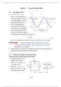
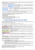
y=Y m cos (ωt+θ) (5.1.1)
where Ym is the amplitude of a Ym
sinusoidal voltage or current, is Ymcos( ) y = Ymcos(t + )
the angular frequency, and is
the phase angle (Figure 5.1.1). t
The time interval between
successive repetitions of the – Ym
same value of y is the period T.
T = 2/
The full range of values of the
Figure 5.1.1
function over a period is a cycle.
The frequency f of repetitions of the function is:
1 ω
f= =
T 2π (5.1.2)
where T is in seconds, f is in cycles per second, or hertz (Hz), and is in rad/s.
Concept An important property of the sinusoidal function is that it is
invariant under linear operations, such as scaling, addition, subtraction,
differentiation, and integration.
Linear operations may change the amplitude and phase of a sinusoidal function but
they do not change its general shape or its frequency.
5.2 Response to Complex Sinusoidal Excitation
Response of RL Circuit to Sinusoidal Excitation
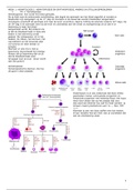
Consider a series RL circuit
+ vR –
supplied from a voltage
source vSRC = Vmcos(t + ),
R
+
as in Figure 5.2.1a.
+ R 2 2L2
vSRC L vL
From KVL: vSRC = vR + vL, – i L
–
where vR = Ri and vL = Ldi/dt.
R
Substituting for these terms:
(a) Figure 5.2.1 (b)
5-1/17
, di
L + Ri=V m cos ( ωt +θ )
dt (5.2.1)
This is a linear, first-order differential equation with a forcing function Vmcos(t + )
on the RHS. The complete solution is the sum of two components:
di
L + Ri=0
A transient component that is the solution to the equation dt , and
which dies out with time. A steady state is assumed to prevail only after the
transient component has become insignificant.
A steady-state component iSS that satisfies Equation 5.2.1. Since the linear
operations on the LHS of Equation 5.2.1 affect the amplitude and phase of iSS
without affecting the frequency. we may consider iSS to be of the form:
i SS =I m cos ( ωt +θ−α ) (5.2.2)
where Im and are unknowns to be determined so as to satisfy Equation 5.2.1.
Substituting iSS from Equation 5.2.2 in Equation 5.2.1:
I m [ −ωL sin ( ωt +θ−α )+ R cos ( ωt +θ−α ) ] =V m cos ( ωt+ θ ) (5.2.3)
If the LHS of Equation 5.2.3 is multiplied and divided by √ R 2+ω2 L2 , it becomes:
I m√ R + ω L −
2 2 2
[ ωL
√ R +ω L
2 2 2
sin ( ωt+θ−α ) +
R
√ R +ω2 L2
2
cos ( ωt +θ−α )
] (5.2.4)
ωL
Let be the angle whose sine is √ R +ω L and whose cosine is therefore
2 2 2
R
√ R2 +ω2 L2 (Figure 5.2.1b). Equation 5.2.4 becomes:
I m √ R2 + ω2 L2 [ −sin β sin ( ωt +θ−α ) +cos β cos ( ωt +θ−α ) ] =V m cos ( ωt +θ )
or:
I m √ R2 + ω2 L2 [ cos ( ωt +θ+ β −α ) ] =V m cos ( ωt +θ ) (5.2.5)
To equalize both sides of Equation 5.2.5 under all conditions, we must have
Vm
I m=
√ R2 + ω2 L2 and = . It follows that:
Vm ωL
i SS= cos ( ωt +θ−α ) tan α=
√ R2 + ω2 L2 , R (5.2.6)
5-2/17
, Response of RL Circuit to Complex Sinusoidal Excitation
Let:
v SRC =V m e j ( ωt +θ )=V m [ cos ( ωt +θ ) + jsin ( ωt +θ ) ] (5.2.7)
Since the circuit is linear, superposition applies, and iSS = iSS1 + iSS2, where iSS1 is the
steady-state response to Vmcos(t + ), as given by Equation 5.2.6, and iSS2 is the
steady-state response to jVmsin(t + ).
The excitation jVmsin(t + ) may be written as
(
jV m cos ωt+θ−
π
)
2 . Hence, iSS2 can
π
be obtained from iss1 by replacing by ( – 2 ) and multiplying Vm by j. This gives:
i SS=
Vm
√ R2+ ω2 L2 [ (
cos ( ωt +θ−α )+ j cos ωt+ θ−α−
π
2 )]
Vm
= [ cos ( ωt+ θ−α ) + j sin ( ωt +θ−α ) ]
√ R 2 +ω 2 L2
Vm j( ωt+θ−α ) ωL
= e tan α=
√R 2 2
+ω L 2
, R (5.2.8)
Concept When a complex sinusoidal excitation vSRC is applied to an LTI
circuit, the response is a complex sinusoidal function whose real part is the
response to the real part of the excitation, Vmcos(t + ), applied alone, and
whose imaginary part is the response to the imaginary part of the excitation,
Vmsin(t + ), applied alone.
In other words, the real and imaginary parts retain their separate identities in linear
operations, without any mutual interaction.
5-3/17
5.1 Sinusoidal Function
y
y=Y m cos (ωt+θ) (5.1.1)
where Ym is the amplitude of a Ym
sinusoidal voltage or current, is Ymcos( ) y = Ymcos(t + )
the angular frequency, and is
the phase angle (Figure 5.1.1). t
The time interval between
successive repetitions of the – Ym
same value of y is the period T.
T = 2/
The full range of values of the
Figure 5.1.1
function over a period is a cycle.
The frequency f of repetitions of the function is:
1 ω
f= =
T 2π (5.1.2)
where T is in seconds, f is in cycles per second, or hertz (Hz), and is in rad/s.
Concept An important property of the sinusoidal function is that it is
invariant under linear operations, such as scaling, addition, subtraction,
differentiation, and integration.
Linear operations may change the amplitude and phase of a sinusoidal function but
they do not change its general shape or its frequency.
5.2 Response to Complex Sinusoidal Excitation
Response of RL Circuit to Sinusoidal Excitation
Consider a series RL circuit
+ vR –
supplied from a voltage
source vSRC = Vmcos(t + ),
R
+
as in Figure 5.2.1a.
+ R 2 2L2
vSRC L vL
From KVL: vSRC = vR + vL, – i L
–
where vR = Ri and vL = Ldi/dt.
R
Substituting for these terms:
(a) Figure 5.2.1 (b)
5-1/17
, di
L + Ri=V m cos ( ωt +θ )
dt (5.2.1)
This is a linear, first-order differential equation with a forcing function Vmcos(t + )
on the RHS. The complete solution is the sum of two components:
di
L + Ri=0
A transient component that is the solution to the equation dt , and
which dies out with time. A steady state is assumed to prevail only after the
transient component has become insignificant.
A steady-state component iSS that satisfies Equation 5.2.1. Since the linear
operations on the LHS of Equation 5.2.1 affect the amplitude and phase of iSS
without affecting the frequency. we may consider iSS to be of the form:
i SS =I m cos ( ωt +θ−α ) (5.2.2)
where Im and are unknowns to be determined so as to satisfy Equation 5.2.1.
Substituting iSS from Equation 5.2.2 in Equation 5.2.1:
I m [ −ωL sin ( ωt +θ−α )+ R cos ( ωt +θ−α ) ] =V m cos ( ωt+ θ ) (5.2.3)
If the LHS of Equation 5.2.3 is multiplied and divided by √ R 2+ω2 L2 , it becomes:
I m√ R + ω L −
2 2 2
[ ωL
√ R +ω L
2 2 2
sin ( ωt+θ−α ) +
R
√ R +ω2 L2
2
cos ( ωt +θ−α )
] (5.2.4)
ωL
Let be the angle whose sine is √ R +ω L and whose cosine is therefore
2 2 2
R
√ R2 +ω2 L2 (Figure 5.2.1b). Equation 5.2.4 becomes:
I m √ R2 + ω2 L2 [ −sin β sin ( ωt +θ−α ) +cos β cos ( ωt +θ−α ) ] =V m cos ( ωt +θ )
or:
I m √ R2 + ω2 L2 [ cos ( ωt +θ+ β −α ) ] =V m cos ( ωt +θ ) (5.2.5)
To equalize both sides of Equation 5.2.5 under all conditions, we must have
Vm
I m=
√ R2 + ω2 L2 and = . It follows that:
Vm ωL
i SS= cos ( ωt +θ−α ) tan α=
√ R2 + ω2 L2 , R (5.2.6)
5-2/17
, Response of RL Circuit to Complex Sinusoidal Excitation
Let:
v SRC =V m e j ( ωt +θ )=V m [ cos ( ωt +θ ) + jsin ( ωt +θ ) ] (5.2.7)
Since the circuit is linear, superposition applies, and iSS = iSS1 + iSS2, where iSS1 is the
steady-state response to Vmcos(t + ), as given by Equation 5.2.6, and iSS2 is the
steady-state response to jVmsin(t + ).
The excitation jVmsin(t + ) may be written as
(
jV m cos ωt+θ−
π
)
2 . Hence, iSS2 can
π
be obtained from iss1 by replacing by ( – 2 ) and multiplying Vm by j. This gives:
i SS=
Vm
√ R2+ ω2 L2 [ (
cos ( ωt +θ−α )+ j cos ωt+ θ−α−
π
2 )]
Vm
= [ cos ( ωt+ θ−α ) + j sin ( ωt +θ−α ) ]
√ R 2 +ω 2 L2
Vm j( ωt+θ−α ) ωL
= e tan α=
√R 2 2
+ω L 2
, R (5.2.8)
Concept When a complex sinusoidal excitation vSRC is applied to an LTI
circuit, the response is a complex sinusoidal function whose real part is the
response to the real part of the excitation, Vmcos(t + ), applied alone, and
whose imaginary part is the response to the imaginary part of the excitation,
Vmsin(t + ), applied alone.
In other words, the real and imaginary parts retain their separate identities in linear
operations, without any mutual interaction.
5-3/17