Introduction to Research in Marketing
Week 1
What you observe = true value + sampling error + measurement error + statistical error
If any of these are incorrect, your results will be biased, and your recommendations will be
wrong.
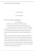
The sample can be made closer to the population by using post-strati cation weights.
Measurement scales
Non-metric scales:
- Nominal
o Number serves only as a label or tag for identifying or classifying objects in
mutually exclusive (can’t be both at the same time) and collectively exhaustive
categories (at least one).
E.g., country, gender.
- Ordinal
o Numbers are assigned to objects to indicate the relative positions of some
characteristic of objects, but not the magnitude of difference between them.
E.g., gold, silver, bronze.
These outcomes can be categorical (labels) or directional (can measure only the direction of
the response, yes/no).
Metric scales:
- Interval
o Numbers are assigned to objects to indicate the relative positions of some
characteristic of objects with differences between objects being comparable;
zero point is arbitrary.
E.g., temperature.
- Ratio
o The most precise scale; absolute zero point. Has all the advantages of other
scales.
E.g., age, weight, height.
When scales are continuous they not only measure direction or
classi cation, but intensity as well (e.g., strongly agree or somewhat
degree).
Some variables are easier to measure than others. Variables such
as attitudes, feelings, or beliefs are more abstract than variables
such as age or income. In that case, more than one question is
needed to capture all facets and reduce measurement error.
Validity: does it measure what it’s supposed to?
Reliability: is it stable?
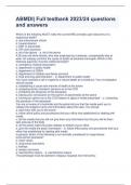
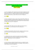
Two possible outcomes of hypothesis testing:
, - Fail to reject the null hypothesis (null is true).
- Reject the null hypothesis (alternative is true).
Upper left corner means how speci c you can be about your
conclusion. Lower right corner is the power of your test.
Two types of error when hypothesis testing:
Type I error: false positive
Type II error: false negative
P-value is the probability of the observed deviation given
that the null hypothesis is true.
- If its low, then the data are unlikely according to the
null, and you can reject the null (low chance of type I
error)
- The threshold is typically set at .05.
- Consider p-values along with interpretation (do the results make sense), power,
measurement, study design (sampling), numerical and graphical summaries of the
data.
Visualization of data:
- To explore the data, see if there are any problems in the dataset such as missing
values.
- To understand and make sense of the data (“model-free evidence”).
- To communicate the results.
Week 2
Step 1: De ning the objectives
Test if there are differences in the mean of a metric (interval or ratio) dependent variable
across different levels of one or more non-metric (nominal or ordinal) independent variables
(“factors”).
Step 2: Designing the ANOVA
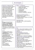
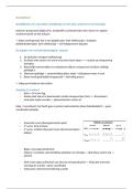
Step 2.1: Interactions.
Designing the ANOVA: think about the model.
Interaction: the effect of one variable on the DV is dependent on
another variable (moderator). (in this case gender)
Use ANOVA to see if there is a “two-way” interaction between
poster and gender.
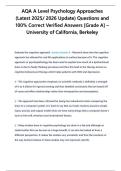
Step 2.2: Using covariates.
Control variables or covariates affect the DV separately from the treatment variables. If
unaccounted for, it may bias the estimates of treatment effects. --> In this case, use ANCOVA.
Covariates/control variables are not included in the design. But, they can affect the results.
, Requirements for control variables:
- Have to be pre-measure (before the outcome): so independent of the treatment.
- There has to be a limited number of control variables.
Control variable in the example is liking of action movies.
Step 3: Checking assumptions.
Step 3.1: Independence. (very important)
Are the observations independent? Affects your estimates and standard errors.
- Between-subjects design: each unit of analysis sees only one combination of IV’s.
o If this is the case, you can generally consider the outcomes to be independent.
o However, omitted control variables can make the outcomes dependent.
- Within-subjects design: each unit of analysis sees all possible treatments.
o Outcomes from the same respondent are obviously correlated.
o We compare each respondent with itself, so control for “luck of the draw”.
o Counterbalance order of the treatments, some respondents see version A rst,
others version C, etc.
o Higher power means that there is more statistical “bang” for fewer subjects.
Repeated-measures ANOVA to control for dependence (not in this
course)
Step 3.2: Equality of variance (homoscedasticity). (somewhat important)
Is the variance equal across treatment groups? Affects your standard errors.
- var(poster A, female) = var(poster B, female) = …
- Perform a Levene’s test. H0 = equal variances (so homoscedasticity), so you want α >
.05, so you can’t reject the null hypothesis. You do not want to reject the null
hypothesis in this case.
- What if homoscedasticity is violated?
o If sample size is about similar across treatment groups, it is less of a problem.
o You can transform the dependent variable (e.g., by using a natural logarithm),
and redo the test.
o You can add a covariate --> ANCOVA, redo the test.
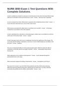
Step 3.3: Normality. (least important)
Are the residuals (approximately) normally distributed? Affects your standard errors only if the
sample is small.
- Residuals (not necessarily the DV) need to be normally distributed.
- Estimate the model rst.
- H0 = normal distribution, so you do not want to reject the null. You want α > .05.
- What is normality is rejected?
o Not a big problem when you have a large sample.
o If you have a small sample: transform the dependent variable (e.g., by using a
natural logarithm) to make the distribution more symmetric.
Week 1
What you observe = true value + sampling error + measurement error + statistical error
If any of these are incorrect, your results will be biased, and your recommendations will be
wrong.
The sample can be made closer to the population by using post-strati cation weights.
Measurement scales
Non-metric scales:
- Nominal
o Number serves only as a label or tag for identifying or classifying objects in
mutually exclusive (can’t be both at the same time) and collectively exhaustive
categories (at least one).
E.g., country, gender.
- Ordinal
o Numbers are assigned to objects to indicate the relative positions of some
characteristic of objects, but not the magnitude of difference between them.
E.g., gold, silver, bronze.
These outcomes can be categorical (labels) or directional (can measure only the direction of
the response, yes/no).
Metric scales:
- Interval
o Numbers are assigned to objects to indicate the relative positions of some
characteristic of objects with differences between objects being comparable;
zero point is arbitrary.
E.g., temperature.
- Ratio
o The most precise scale; absolute zero point. Has all the advantages of other
scales.
E.g., age, weight, height.
When scales are continuous they not only measure direction or
classi cation, but intensity as well (e.g., strongly agree or somewhat
degree).
Some variables are easier to measure than others. Variables such
as attitudes, feelings, or beliefs are more abstract than variables
such as age or income. In that case, more than one question is
needed to capture all facets and reduce measurement error.
Validity: does it measure what it’s supposed to?
Reliability: is it stable?
Two possible outcomes of hypothesis testing:
, - Fail to reject the null hypothesis (null is true).
- Reject the null hypothesis (alternative is true).
Upper left corner means how speci c you can be about your
conclusion. Lower right corner is the power of your test.
Two types of error when hypothesis testing:
Type I error: false positive
Type II error: false negative
P-value is the probability of the observed deviation given
that the null hypothesis is true.
- If its low, then the data are unlikely according to the
null, and you can reject the null (low chance of type I
error)
- The threshold is typically set at .05.
- Consider p-values along with interpretation (do the results make sense), power,
measurement, study design (sampling), numerical and graphical summaries of the
data.
Visualization of data:
- To explore the data, see if there are any problems in the dataset such as missing
values.
- To understand and make sense of the data (“model-free evidence”).
- To communicate the results.
Week 2
Step 1: De ning the objectives
Test if there are differences in the mean of a metric (interval or ratio) dependent variable
across different levels of one or more non-metric (nominal or ordinal) independent variables
(“factors”).
Step 2: Designing the ANOVA
Step 2.1: Interactions.
Designing the ANOVA: think about the model.
Interaction: the effect of one variable on the DV is dependent on
another variable (moderator). (in this case gender)
Use ANOVA to see if there is a “two-way” interaction between
poster and gender.
Step 2.2: Using covariates.
Control variables or covariates affect the DV separately from the treatment variables. If
unaccounted for, it may bias the estimates of treatment effects. --> In this case, use ANCOVA.
Covariates/control variables are not included in the design. But, they can affect the results.
, Requirements for control variables:
- Have to be pre-measure (before the outcome): so independent of the treatment.
- There has to be a limited number of control variables.
Control variable in the example is liking of action movies.
Step 3: Checking assumptions.
Step 3.1: Independence. (very important)
Are the observations independent? Affects your estimates and standard errors.
- Between-subjects design: each unit of analysis sees only one combination of IV’s.
o If this is the case, you can generally consider the outcomes to be independent.
o However, omitted control variables can make the outcomes dependent.
- Within-subjects design: each unit of analysis sees all possible treatments.
o Outcomes from the same respondent are obviously correlated.
o We compare each respondent with itself, so control for “luck of the draw”.
o Counterbalance order of the treatments, some respondents see version A rst,
others version C, etc.
o Higher power means that there is more statistical “bang” for fewer subjects.
Repeated-measures ANOVA to control for dependence (not in this
course)
Step 3.2: Equality of variance (homoscedasticity). (somewhat important)
Is the variance equal across treatment groups? Affects your standard errors.
- var(poster A, female) = var(poster B, female) = …
- Perform a Levene’s test. H0 = equal variances (so homoscedasticity), so you want α >
.05, so you can’t reject the null hypothesis. You do not want to reject the null
hypothesis in this case.
- What if homoscedasticity is violated?
o If sample size is about similar across treatment groups, it is less of a problem.
o You can transform the dependent variable (e.g., by using a natural logarithm),
and redo the test.
o You can add a covariate --> ANCOVA, redo the test.
Step 3.3: Normality. (least important)
Are the residuals (approximately) normally distributed? Affects your standard errors only if the
sample is small.
- Residuals (not necessarily the DV) need to be normally distributed.
- Estimate the model rst.
- H0 = normal distribution, so you do not want to reject the null. You want α > .05.
- What is normality is rejected?
o Not a big problem when you have a large sample.
o If you have a small sample: transform the dependent variable (e.g., by using a
natural logarithm) to make the distribution more symmetric.