Solutions to Exercises in
Introduction to Economic Growth
(Second Edition)
Charles I. Jones
(with Chao Wei and Jesse Czelusta)
Department of Economics
U.C. Berkeley
Berkeley, CA 94720-3880
September 18, 2001
, 1
1 Introduction
No problems.
2 The Solow Model
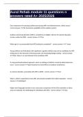
Exercise 1. A decrease in the investment rate.
A decrease in the investment rate causes the sỹ curve to shift down: at any
given level of k̃, the investment-technology ratio is lower at the new rate of sav-
ing/investment.
Assuming the economy began in steady state, the capital-technology ratio is
now higher than is consistent with the reduced saving rate, so it declines gradually,
as shown in Figure 1.
Figure 1: A Decrease in the Investment Rate
~
(n+g+d)k
~
s’y
~
s’’ y
~ ~
k** k*
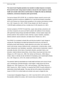
The log of output per worker y evolves as in Figure 2, and the dynamics of
˙
the growth rate are shown in Figure 3. Recall that log ỹ = α log k̃ and k̃/k̃ =
s00 k̃ α−1 − (n + g + d).
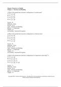
The policy permanently reduces the level of output per worker, but the growth
rate per worker is only temporarily reduced and will return to g in the long run.
, 2
Figure 2: y(t)
LOG y
TIME
Figure 3: Growth Rate of Output per Worker
.
y/ y
g
t* TIME
, 3
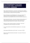
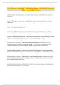
Exercise 2. An increase in the labor force.
The key to this question is to recognize that the initial effect of a sudden in-
crease in the labor force is to reduce the capital-labor ratio since k ≡ K/L and K
is fixed at a moment in time. Assuming the economy was in steady state prior to
the increase in labor force, k falls from k ∗ to some new level k1 . Notice that this is
a movement along the sy and (n + d)k curves rather than a shift of either schedule:
both curves are plotted as functions of k, so that a change in k is a movement along
the curves. (For this reason, it is somewhat tricky to put this question first!)
At k1 , sy > (n + d)k1 , so that k̇ > 0, and the economy evolves according to
the usual Solow dynamics, as shown in Figure 4.
Figure 4: An Increase in the Labor Force
(n + d) k
sy
k1 k* k
In the short run, per capita output and capital drop in response to a inlarge flow
of workers. Then these two variables start to grow (at a decreasing rate), until in
the long run per capita capital returns to the original level, k ∗ . In the long run,
nothing has changed!
Exercise 3. An income tax.
Assume that the government throws away the resources it receives in taxes.
Then an income tax reduces the total amount available for investing and shifts the
investment curve down as shown in Figure 5.
Introduction to Economic Growth
(Second Edition)
Charles I. Jones
(with Chao Wei and Jesse Czelusta)
Department of Economics
U.C. Berkeley
Berkeley, CA 94720-3880
September 18, 2001
, 1
1 Introduction
No problems.
2 The Solow Model
Exercise 1. A decrease in the investment rate.
A decrease in the investment rate causes the sỹ curve to shift down: at any
given level of k̃, the investment-technology ratio is lower at the new rate of sav-
ing/investment.
Assuming the economy began in steady state, the capital-technology ratio is
now higher than is consistent with the reduced saving rate, so it declines gradually,
as shown in Figure 1.
Figure 1: A Decrease in the Investment Rate
~
(n+g+d)k
~
s’y
~
s’’ y
~ ~
k** k*
The log of output per worker y evolves as in Figure 2, and the dynamics of
˙
the growth rate are shown in Figure 3. Recall that log ỹ = α log k̃ and k̃/k̃ =
s00 k̃ α−1 − (n + g + d).
The policy permanently reduces the level of output per worker, but the growth
rate per worker is only temporarily reduced and will return to g in the long run.
, 2
Figure 2: y(t)
LOG y
TIME
Figure 3: Growth Rate of Output per Worker
.
y/ y
g
t* TIME
, 3
Exercise 2. An increase in the labor force.
The key to this question is to recognize that the initial effect of a sudden in-
crease in the labor force is to reduce the capital-labor ratio since k ≡ K/L and K
is fixed at a moment in time. Assuming the economy was in steady state prior to
the increase in labor force, k falls from k ∗ to some new level k1 . Notice that this is
a movement along the sy and (n + d)k curves rather than a shift of either schedule:
both curves are plotted as functions of k, so that a change in k is a movement along
the curves. (For this reason, it is somewhat tricky to put this question first!)
At k1 , sy > (n + d)k1 , so that k̇ > 0, and the economy evolves according to
the usual Solow dynamics, as shown in Figure 4.
Figure 4: An Increase in the Labor Force
(n + d) k
sy
k1 k* k
In the short run, per capita output and capital drop in response to a inlarge flow
of workers. Then these two variables start to grow (at a decreasing rate), until in
the long run per capita capital returns to the original level, k ∗ . In the long run,
nothing has changed!
Exercise 3. An income tax.
Assume that the government throws away the resources it receives in taxes.
Then an income tax reduces the total amount available for investing and shifts the
investment curve down as shown in Figure 5.