HT5 Macroecons (Economic Growth)
Week's outline
Exogenous (Solow-Swan) and endogenous (Romer-Jones) growth
Directed technological change and income inequality
Empirical evidence, policy considerations, extensions
Lecture 12: Growth models—Solow, Romer, Jones
Introduction to Growth
What is growth?
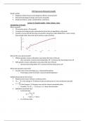
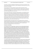
US economy grows ~2% annually
Constant percentage growth represented as linear line on logarithmic scale graph
Growth is concerned with the long-run growth at long time scales (dotted line, x-axis is a long
time period) rather than short term business cycles (red line)
o
Why do We Care about Growth?
Without growth, resource allocation is just about the share of the pie
o Zero sum game: someone becoming better off ⇒ someone else becoming worse off
With growth, resource allocation is also about the size of the pie
o Someone becoming better off ≠ someone else becoming worse off
Where does growth come from?
Growth comes from technology (e.g., Industrial Revolution)
o Technology comes from ideas, research and development
Mathematical tools for the lecture
Models in this lecture will be in continuous time
𝑋𝑡+1 − 𝑋𝑡 is the change in 𝑋 between today and tomorrow (or next month/year/decade)
is the change in 𝑋 between now and the instant immediately after
o Formally, it is (𝑋𝑡+Δ − 𝑋𝑡)/Δ as Δ → 0, hence the derivative
Definitions of growth rates
o In discrete time
o In continuous time
,
(By the chain rule, see appendix for derivation)
The Solow Model
Setup
Distilled from Swan (1956) and Solow (1957)
o Growth exogenously comes from technology and/or population
o Not many knobs or levers are available for policymakers, but still ground-breaking in
showing us where to look for growth
Production function: GDP is produced with three inputs- capital, labour and labour-augmenting
tech
o Monotonicity: If any three inputs increase, GDP increases
o Concavity: Production features diminishing returns for each input
o Constant returns to scale: doubling inputs results in doubling GDP
Industrial interpretation: the following are equivalent
Making one production facility twice as large
Replicating one production facility elsewhere
o The Cobb-Douglas form is mathematically convenient, but not necessary as long as the
properties above hold
o Empirical estimates: 𝛼 is roughly between 0.3 and 0.4
Law of motion of capital: change in capital over time driven by investment and depreciation
(proportional to capital stock level)
o Capital can only be increased by active investment
o Capital can only be decreased by passive depreciation
Existing physical capital cannot be actively reclaimed
Depreciated capital is destroyed: it cannot be reused/recycled
o We assume 𝛿 ∈ (0, 1)
o In Mathematics, this is an Ordinary Differential Equation (ODE)
𝐾𝑡 can be written as 𝐾(𝑡)
K̇ t can be written as 𝐾′(𝑡)
A differential equation involves functions and their derivatives
Solution: a function that satisfies the equation
o Empirical estimates: 𝛿 is about 3% yearly
Investment rule: investment level is a constant fraction (s) of output
, o How exactly savings are directed to investment is not important, we just assume they
are
o The remaining fraction (1 − 𝑠) is spent on consumption
o It can be micro-founded (derived in microeconomics) if intertemporal utility function is
log-additive
o Proportion 𝑠 can be affected by policy (e.g., VAT)
o Important: 𝑠 is the marginal propensity to save, not the average savings rate (here
they’re assumed to coincide)
Resource constraint: GDP is either consumed or invested
o Equivalent to closed economy national accounting, disregarding government spending
o It can be microfounded: equilibrium version of the budget constraint of a household
facing a consumption-savings problem
Population and technology grow at a constant percentage rate per period
o Exogenous and constant net growth rate 𝑔𝐿 and 𝑔𝐴, assumed to be ∈ [0, 1]
o 𝑔𝐿 can be affected by policy (e.g., fertility policies)
o 𝑔𝐴 can be affected by policy (e.g., R&D subsidies, but also see Romer’s model)
o But it does not explain the source of growth
Steady state growth
Naïve definition of steady state: K̇ t =0
o Solving with this definition:
𝐼𝑡 = 𝛿𝐾𝑡 = 𝑠𝑌𝑡.
𝑌𝑡 = 𝛿𝐾𝑡/𝑠 = 𝐾𝑡𝛼(𝐴𝑡𝐿𝑡)1−𝛼.
𝐾𝑡1−𝛼 = (𝑠/𝛿)(𝐴𝑡𝐿𝑡)1−𝛼.
Solution:
o But 𝐴𝑡 and 𝐿𝑡 grow, so K also grows (going against the initial assumption). This violates
the naïve definition of steady state
This model does not have a steady state in physical (and absolute) units
o We need to express variables relative to exogenously growing variables 𝐴𝑡 and 𝐿𝑡
o We focus on 𝑘𝑡:= 𝐾𝑡/(𝐴𝑡𝐿𝑡), i.e., capital per effective unit of labour
o Resulting definition of steady state: k˙ t=0
o Key: 𝐾𝑡 in the steady state will grow matching the pace of 𝐴𝑡 and 𝐿𝑡
o Interpretation: whether 𝐾𝑡 is “big” or “small” depends on tech and population
o Key for some intuition: 𝐾𝑡/𝐿𝑡 known as capital depth (how much capital each worker
uses in production)
Generalised notion of steady-state: achieving time-invariant growth rates in the steady state
o GDP grows at a constant rate driven by 𝑔𝐿 and 𝑔𝐴.
Intensive form of the Solow model
Define 𝑥𝑡 := 𝑋𝑡/(𝐴𝑡𝐿𝑡) for each 𝑋𝑡 ∈ {𝑌𝑡, 𝐼𝑡, 𝐶𝑡, 𝐾𝑡} and rewrite the model
,
o Law of motion:
Derive by solving
Intuitively, 𝑘𝑡 decreases as 𝐴𝑡 and 𝐿𝑡 increases, so you should factor in 𝑔𝐴
and 𝑔𝐿 in addition to depreciation
o The rest of the equations can be easily obtained by dividing both sides by (𝐴𝑡𝐿𝑡)
Steady state: k˙ t=0
o Solving: 𝑖𝑡 = (𝑔𝐴 + 𝑔𝐿 + 𝛿)𝑘𝑡 = 𝑠𝑦𝑡 = 𝑠𝑘𝛼.
o Hence, 𝑠𝑘𝛼 = (𝑔𝐴 + 𝑔𝐿 + 𝛿)𝑘
o In words, investment = “depreciation”
o Rearranging, we obtain:
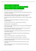
Phase Diagram and steady state
A phase diagram shows how the state of a dynamical system changes depending on, e.g.,
functional forms and parameter values
Phase Diagram
o
o Vertical axis: y, 𝑐, 𝑖
o Horizontal axis: 𝑘𝑡
o Curves on the graph
Week's outline
Exogenous (Solow-Swan) and endogenous (Romer-Jones) growth
Directed technological change and income inequality
Empirical evidence, policy considerations, extensions
Lecture 12: Growth models—Solow, Romer, Jones
Introduction to Growth
What is growth?
US economy grows ~2% annually
Constant percentage growth represented as linear line on logarithmic scale graph
Growth is concerned with the long-run growth at long time scales (dotted line, x-axis is a long
time period) rather than short term business cycles (red line)
o
Why do We Care about Growth?
Without growth, resource allocation is just about the share of the pie
o Zero sum game: someone becoming better off ⇒ someone else becoming worse off
With growth, resource allocation is also about the size of the pie
o Someone becoming better off ≠ someone else becoming worse off
Where does growth come from?
Growth comes from technology (e.g., Industrial Revolution)
o Technology comes from ideas, research and development
Mathematical tools for the lecture
Models in this lecture will be in continuous time
𝑋𝑡+1 − 𝑋𝑡 is the change in 𝑋 between today and tomorrow (or next month/year/decade)
is the change in 𝑋 between now and the instant immediately after
o Formally, it is (𝑋𝑡+Δ − 𝑋𝑡)/Δ as Δ → 0, hence the derivative
Definitions of growth rates
o In discrete time
o In continuous time
,
(By the chain rule, see appendix for derivation)
The Solow Model
Setup
Distilled from Swan (1956) and Solow (1957)
o Growth exogenously comes from technology and/or population
o Not many knobs or levers are available for policymakers, but still ground-breaking in
showing us where to look for growth
Production function: GDP is produced with three inputs- capital, labour and labour-augmenting
tech
o Monotonicity: If any three inputs increase, GDP increases
o Concavity: Production features diminishing returns for each input
o Constant returns to scale: doubling inputs results in doubling GDP
Industrial interpretation: the following are equivalent
Making one production facility twice as large
Replicating one production facility elsewhere
o The Cobb-Douglas form is mathematically convenient, but not necessary as long as the
properties above hold
o Empirical estimates: 𝛼 is roughly between 0.3 and 0.4
Law of motion of capital: change in capital over time driven by investment and depreciation
(proportional to capital stock level)
o Capital can only be increased by active investment
o Capital can only be decreased by passive depreciation
Existing physical capital cannot be actively reclaimed
Depreciated capital is destroyed: it cannot be reused/recycled
o We assume 𝛿 ∈ (0, 1)
o In Mathematics, this is an Ordinary Differential Equation (ODE)
𝐾𝑡 can be written as 𝐾(𝑡)
K̇ t can be written as 𝐾′(𝑡)
A differential equation involves functions and their derivatives
Solution: a function that satisfies the equation
o Empirical estimates: 𝛿 is about 3% yearly
Investment rule: investment level is a constant fraction (s) of output
, o How exactly savings are directed to investment is not important, we just assume they
are
o The remaining fraction (1 − 𝑠) is spent on consumption
o It can be micro-founded (derived in microeconomics) if intertemporal utility function is
log-additive
o Proportion 𝑠 can be affected by policy (e.g., VAT)
o Important: 𝑠 is the marginal propensity to save, not the average savings rate (here
they’re assumed to coincide)
Resource constraint: GDP is either consumed or invested
o Equivalent to closed economy national accounting, disregarding government spending
o It can be microfounded: equilibrium version of the budget constraint of a household
facing a consumption-savings problem
Population and technology grow at a constant percentage rate per period
o Exogenous and constant net growth rate 𝑔𝐿 and 𝑔𝐴, assumed to be ∈ [0, 1]
o 𝑔𝐿 can be affected by policy (e.g., fertility policies)
o 𝑔𝐴 can be affected by policy (e.g., R&D subsidies, but also see Romer’s model)
o But it does not explain the source of growth
Steady state growth
Naïve definition of steady state: K̇ t =0
o Solving with this definition:
𝐼𝑡 = 𝛿𝐾𝑡 = 𝑠𝑌𝑡.
𝑌𝑡 = 𝛿𝐾𝑡/𝑠 = 𝐾𝑡𝛼(𝐴𝑡𝐿𝑡)1−𝛼.
𝐾𝑡1−𝛼 = (𝑠/𝛿)(𝐴𝑡𝐿𝑡)1−𝛼.
Solution:
o But 𝐴𝑡 and 𝐿𝑡 grow, so K also grows (going against the initial assumption). This violates
the naïve definition of steady state
This model does not have a steady state in physical (and absolute) units
o We need to express variables relative to exogenously growing variables 𝐴𝑡 and 𝐿𝑡
o We focus on 𝑘𝑡:= 𝐾𝑡/(𝐴𝑡𝐿𝑡), i.e., capital per effective unit of labour
o Resulting definition of steady state: k˙ t=0
o Key: 𝐾𝑡 in the steady state will grow matching the pace of 𝐴𝑡 and 𝐿𝑡
o Interpretation: whether 𝐾𝑡 is “big” or “small” depends on tech and population
o Key for some intuition: 𝐾𝑡/𝐿𝑡 known as capital depth (how much capital each worker
uses in production)
Generalised notion of steady-state: achieving time-invariant growth rates in the steady state
o GDP grows at a constant rate driven by 𝑔𝐿 and 𝑔𝐴.
Intensive form of the Solow model
Define 𝑥𝑡 := 𝑋𝑡/(𝐴𝑡𝐿𝑡) for each 𝑋𝑡 ∈ {𝑌𝑡, 𝐼𝑡, 𝐶𝑡, 𝐾𝑡} and rewrite the model
,
o Law of motion:
Derive by solving
Intuitively, 𝑘𝑡 decreases as 𝐴𝑡 and 𝐿𝑡 increases, so you should factor in 𝑔𝐴
and 𝑔𝐿 in addition to depreciation
o The rest of the equations can be easily obtained by dividing both sides by (𝐴𝑡𝐿𝑡)
Steady state: k˙ t=0
o Solving: 𝑖𝑡 = (𝑔𝐴 + 𝑔𝐿 + 𝛿)𝑘𝑡 = 𝑠𝑦𝑡 = 𝑠𝑘𝛼.
o Hence, 𝑠𝑘𝛼 = (𝑔𝐴 + 𝑔𝐿 + 𝛿)𝑘
o In words, investment = “depreciation”
o Rearranging, we obtain:
Phase Diagram and steady state
A phase diagram shows how the state of a dynamical system changes depending on, e.g.,
functional forms and parameter values
Phase Diagram
o
o Vertical axis: y, 𝑐, 𝑖
o Horizontal axis: 𝑘𝑡
o Curves on the graph