Week 1
Deep learning is based on the approach of having many hierarchy levels. The hierarchy of
concepts enable the computer to learn complicated concepts by building them out of simpler
ones.
A computer can reason automatically about statements in formal languages using logical
inference rules. This is known as the knowledge base approach to AI.
AI systems need the ability to acquire their own knowledge by extracting patterns from raw data.
This capability is known as machine learning.
The performance of simple machine learning algorithms depends heavily on the representation of
the data they are given.
Each piece of information included in the representation is known as a feature.
Representation learning: Use machine learning to discover not only the mapping from
representation to output but also the representation itself.
- Learned representations often result in much better performance than can be obtained with
hand designed representations.
- Auto-encoder is the combination of an encoder function and a decoder function
When designing features or algorithms for learning features, our goal is usually to separate the
factors of variation that explain the observed data.
- Most applications require us to disentangle the factors of variation and discard the ones that
we do not care about.
Deep learning solves the central problem of obtaining representations in representation learning
by introducing representations that are expressed in terms of other, simpler representations.
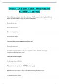
- The quintessential example of a deep learning model is the feedforward deep network, or
multi later perceptron (MLP). A multilayer perceptron is just a mathematical function mapping
some set of input values to output values. The function is formed by composing many
simpler functions.
Visible layer: contains the variables that we are able to observe.
Hidden layers: extract increasingly abstract features.
- Values are not given in the data, instead the models must determine which concepts are
useful for explaining the relationships in the observed data.
For machine learning you have features x which are used to make predictions y.̂
Labels are what you want to predict.
Features are the variables you use to make the prediction. They make up the representation.
,The objective of regression: we want to predict a continuous output value (scalar), given an input
vector.
- ŷ = f (x; w)
- ŷ = prediction
- f = regression function
- x = input vector
- W = paramaters to learn
- Input is transformed using parameters
Linear regression:
- ŷ = f (x; w) = x T w
- T represents dot product, number of parameters == number of features
- We want the weighted sum of the parameters. This is done by taking the dot product of the
vectors.
Weights and biases:
- If the input is a vector of zeros x = [0,0,0… . ]T the output is always 0.
- To overcome this we add bias (also known as an intercept)
- X = [x,1]
- W = [w,b]
- So we always have one more parameter to learn.
- Bias is an extra parameter that we always get, it is the same for all datapoints.
Goodness of t: given a machine learning model, how good is it. We measure that and give it a
score.
- Typically measure the di erence between the ground truth and the prediction.
- Loss function: (yn − yn̂ )2
1
(yn − xnT w)2
- Learning objective (SSE):
2 ∑
- xnT w == yn̂
- The equation is squared to punish bigger mistakes/di erences
Linear regression forward and loss: parameters are needed to compute the loss, while the loss is
needed to know how well the parameters perform.
The best parameters W are the ones with the lowest sum of squared errors (SSE).
fi ff ff
, To nd the minimum SSE, we need to take the derivative of the SEE and set it to zero.
1
(yn − xnT w)2 becomes:
- s(w) =
2 ∑
d
(yn − xnT w)xn (derivative)
∑
- (s w) = −
dw
d
- We transform it to vecoterised form: s(w) = − (y − w T x)x T
dw
- Setting the derivative to 0 gives: −(y − w T x)x T = 0
- Solving this gives: w = (x x T )−1 * x y T
Linear regression can be solved in one equation. Unfortunately most machine learning models
cannot be solved this directly. Most problems have more than 1 (non-convex) minimum so then
the mathematical approach from before does not work.
Gradient descent:
- Slow iterative way to get the nearest minimum
- The gradient tells use the slope of a function
- Greedy approach
- Useful when non-convex
- Step by step guide:
1. Initialise parameters randomly
2. Take gradient and update parameters (keep taking new parameters and taking the
gradient until minimum is found)
3. Stop when at a minimum and can’t go lower. Meaning new step is not better than
previous step.
Regression is nothing more than nding those parameters that minimise our squared errors.
Parameters are values that we need to learn.
Hyper parameters are parameters that we would like to learn but unfortunately cannot learn, so
then we have to set them.
Learning rate (lambda) λ is an important hyper parameter.
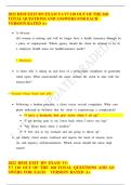
Setting the step size in gradient descent:
- Too low, a small learning rate requires many updates before reaching the minimum point.
- Just right, the optimal learning rate swiftly reaches the minimum point
- Too high, too large learning rate causes drastic updates which lead to divergent behaviours
and overshooting the minimum.
fi fi
, Stochastic gradient descent:
- Go over subsets of examples, compute gradient for subset and update.
- Solves problem of going over all samples with gradient descent.
Linear regressions is a one layer network with:
- Forward propagation: compute ŷ = w T x
- Backward propagation: compute gradient of x
1 2
- Loss: square di erence (y − y)̂ , gradient (y − y)̂
2
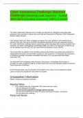
Polynomial regression:
- New forward function: ŷ = w T x + w T (x 2) + . . . + w T (x n)
- The higher the value of n, the more non-linear the regression function.
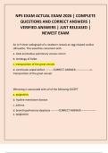
You can solve over tting by adding more data, but this does require a lot of data.
Tackling over tting with Regularisation:
- Data point xn
- True value yn
- Predicted value ŷ = f (x n : w)
1
(yn − w T xn)2 + λ R(w)
2∑
Learning objective: min
-
n
- λ is a hyperparameter (learning rate)
2
- With R(w) = ∑ wd
d
- The lower the values of the weights the lower the error.
- Intuition: high weights are key factors in over tting
- Find a balance between t and complexity
- Using only R(w) would result in value 0 for w being the best option
- It involves adding a penalty term to the model's optimization objective, discouraging overly
complex models by penalizing large parameter values or high complexity.
fi ff fi fi fi
Deep learning is based on the approach of having many hierarchy levels. The hierarchy of
concepts enable the computer to learn complicated concepts by building them out of simpler
ones.
A computer can reason automatically about statements in formal languages using logical
inference rules. This is known as the knowledge base approach to AI.
AI systems need the ability to acquire their own knowledge by extracting patterns from raw data.
This capability is known as machine learning.
The performance of simple machine learning algorithms depends heavily on the representation of
the data they are given.
Each piece of information included in the representation is known as a feature.
Representation learning: Use machine learning to discover not only the mapping from
representation to output but also the representation itself.
- Learned representations often result in much better performance than can be obtained with
hand designed representations.
- Auto-encoder is the combination of an encoder function and a decoder function
When designing features or algorithms for learning features, our goal is usually to separate the
factors of variation that explain the observed data.
- Most applications require us to disentangle the factors of variation and discard the ones that
we do not care about.
Deep learning solves the central problem of obtaining representations in representation learning
by introducing representations that are expressed in terms of other, simpler representations.
- The quintessential example of a deep learning model is the feedforward deep network, or
multi later perceptron (MLP). A multilayer perceptron is just a mathematical function mapping
some set of input values to output values. The function is formed by composing many
simpler functions.
Visible layer: contains the variables that we are able to observe.
Hidden layers: extract increasingly abstract features.
- Values are not given in the data, instead the models must determine which concepts are
useful for explaining the relationships in the observed data.
For machine learning you have features x which are used to make predictions y.̂
Labels are what you want to predict.
Features are the variables you use to make the prediction. They make up the representation.
,The objective of regression: we want to predict a continuous output value (scalar), given an input
vector.
- ŷ = f (x; w)
- ŷ = prediction
- f = regression function
- x = input vector
- W = paramaters to learn
- Input is transformed using parameters
Linear regression:
- ŷ = f (x; w) = x T w
- T represents dot product, number of parameters == number of features
- We want the weighted sum of the parameters. This is done by taking the dot product of the
vectors.
Weights and biases:
- If the input is a vector of zeros x = [0,0,0… . ]T the output is always 0.
- To overcome this we add bias (also known as an intercept)
- X = [x,1]
- W = [w,b]
- So we always have one more parameter to learn.
- Bias is an extra parameter that we always get, it is the same for all datapoints.
Goodness of t: given a machine learning model, how good is it. We measure that and give it a
score.
- Typically measure the di erence between the ground truth and the prediction.
- Loss function: (yn − yn̂ )2
1
(yn − xnT w)2
- Learning objective (SSE):
2 ∑
- xnT w == yn̂
- The equation is squared to punish bigger mistakes/di erences
Linear regression forward and loss: parameters are needed to compute the loss, while the loss is
needed to know how well the parameters perform.
The best parameters W are the ones with the lowest sum of squared errors (SSE).
fi ff ff
, To nd the minimum SSE, we need to take the derivative of the SEE and set it to zero.
1
(yn − xnT w)2 becomes:
- s(w) =
2 ∑
d
(yn − xnT w)xn (derivative)
∑
- (s w) = −
dw
d
- We transform it to vecoterised form: s(w) = − (y − w T x)x T
dw
- Setting the derivative to 0 gives: −(y − w T x)x T = 0
- Solving this gives: w = (x x T )−1 * x y T
Linear regression can be solved in one equation. Unfortunately most machine learning models
cannot be solved this directly. Most problems have more than 1 (non-convex) minimum so then
the mathematical approach from before does not work.
Gradient descent:
- Slow iterative way to get the nearest minimum
- The gradient tells use the slope of a function
- Greedy approach
- Useful when non-convex
- Step by step guide:
1. Initialise parameters randomly
2. Take gradient and update parameters (keep taking new parameters and taking the
gradient until minimum is found)
3. Stop when at a minimum and can’t go lower. Meaning new step is not better than
previous step.
Regression is nothing more than nding those parameters that minimise our squared errors.
Parameters are values that we need to learn.
Hyper parameters are parameters that we would like to learn but unfortunately cannot learn, so
then we have to set them.
Learning rate (lambda) λ is an important hyper parameter.
Setting the step size in gradient descent:
- Too low, a small learning rate requires many updates before reaching the minimum point.
- Just right, the optimal learning rate swiftly reaches the minimum point
- Too high, too large learning rate causes drastic updates which lead to divergent behaviours
and overshooting the minimum.
fi fi
, Stochastic gradient descent:
- Go over subsets of examples, compute gradient for subset and update.
- Solves problem of going over all samples with gradient descent.
Linear regressions is a one layer network with:
- Forward propagation: compute ŷ = w T x
- Backward propagation: compute gradient of x
1 2
- Loss: square di erence (y − y)̂ , gradient (y − y)̂
2
Polynomial regression:
- New forward function: ŷ = w T x + w T (x 2) + . . . + w T (x n)
- The higher the value of n, the more non-linear the regression function.
You can solve over tting by adding more data, but this does require a lot of data.
Tackling over tting with Regularisation:
- Data point xn
- True value yn
- Predicted value ŷ = f (x n : w)
1
(yn − w T xn)2 + λ R(w)
2∑
Learning objective: min
-
n
- λ is a hyperparameter (learning rate)
2
- With R(w) = ∑ wd
d
- The lower the values of the weights the lower the error.
- Intuition: high weights are key factors in over tting
- Find a balance between t and complexity
- Using only R(w) would result in value 0 for w being the best option
- It involves adding a penalty term to the model's optimization objective, discouraging overly
complex models by penalizing large parameter values or high complexity.
fi ff fi fi fi