Summary Applied Multivariate Data Analysis
Important Analyses
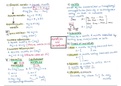
Linear Regression – a linear regression is a way of predicting values of one variable from
another based on a model that describes a straight line. This line summarizes the pattern of
the data best.
- R2 – explained variance of the model, proportion of variance in the outcome variable
that is shared by the predictor variable
- F – ratio of how much variability the model can explain relative to how much it can’t
explain
- b-value – the gradient of the line and the strength of the relationship between a
predictor and the outcome variable
b0 = intercept, the value of the outcome variable we would predict if the
predictor value would be 0
b-coefficients vs. beta-coefficients
- b = change in outcome is associated with a unit change in the predictor
- beta = the same as b-value, but expressed as standad deviations. Thus, because
these values are standardized we can compare them across studies or multiple
predictors when you have a multiple regression
How good is the model?
- If the regression model can predict something, it will be more steep than the flat line
that would be the mean of all people on the dependent variable
- If the F-value is greater than 1, it means the model can explain some variance
F = 100: there is a 100 times more explained variance than unexplained variance
F = 1: explained and unexplained variance is the same
- In order to check how well the model fits the data, we check multiple things:
Standardized residuals/residual distance – for cases with a large prediction error
Distance from the individual points to the regression line (the model)
Influential cases that might bias the regression model do not have large
residuals per se > why we also check for other distances
Mahalanobis distance – for outlying cases on the predictor
Distance that the individual point is removed from the other points in the
space of the independent variables (thus, on the x-axis)
Cook’s distance – for unfluential cases, measures the influence of a single case on
the model as a whole
How much does the regression slope shift due to inclusion of this outlier
,General rules to see if there is an outlier based on standardized residuals:
1. Standardized residuals with an absolute greater value than 3.29 (approximately 3) is
cause for concern
2. If more than 1% of the sample cases have a residual above 2.58 (approximately 2.5) it
is cause for concern
3. If more than 5% of the sample cases have a residual above 1.96 (approximately 2) it is
cause for concern
General rules to see if there is an outlier based on the Mahalanobis distance:
1. Influential cases have values above 25 in large samples (500 or more)
2. Influential cases have values above 15 in smaller samples (100)
3. Influential cases have values above 11 in small samples (30 or less)
Multiple regression – this is the same as a simple linear regression, but with multiple
predictors.
- Ideally, all predictors have a high correlation with the outcome variable but the
correlations among the predictors is low. The higher the correlation among
predictors, the less information each predictor adds uniquely
- When the correlation among predictors is high, it causes multicollinearity: this
means that the variables basically explain the same variance (at least for a large
part). SPSS automatically corrects for this, which can cause changes between the
regression coefficient and the correlations (e.g. there is a positive correlation yet the
regression coefficient is negative). This is called bouncing betas
- Ways to detect multicollinearity:
1. Correlations between predictors is higher than .80
2. VIF of a predictor > 10
3. Tolerance of a predictor < .10
- Apart from bouncing betas, multicollinearity also causes other problems, namely, a
limited size of R given the number of predictors (adding a predictor with little unique
contribution) and difficulties with determining the importance of predictors (refers to
bouncing betas)
Assumptions Regression Analysis
1. Linearity – the relationship between the predictor and the outcome variable must be
linear
Check 1) residual plot with Zpred. X vs. Zresid. Y or 2) scatterplot with predictor X
vs. dependent variable Y
If the residuals show a curved pattern, the regression model is not optimal >
assumption is not met
2. Homoscedasticity / homogeneity of variance – for each value of the predictors, the
variance of the residuals should be equal (or: spread of outcome scores is roughly
equal at different points in the predictor variable)
Check the residual plot with Zpred. X vs. Zresid. Y
The residuals should al be equally centered around 0, with generally an equal
amount of residuals an all sides (left, right, under and above). If this is not the
case, we call it heteroscedasticity
, If the residuals increase with the predicted values, the heteroscedasticity may be
explained with another predictor
3. Normally distributed errors – if the errors are not normally distributed, we cannot
trust the –values of the significance tests (with small N)
Check 1) histogram of the residuals for multiple peaks or outliers or 2) scatterplot
with Zpred. X and Zresid. Y for the normal curve or 3) Q-Q plots
4. Independence of errors – all values of the outcome variable should come from a
different person
Error terms of observations should be uncorrelated
Important Analyses
Linear Regression – a linear regression is a way of predicting values of one variable from
another based on a model that describes a straight line. This line summarizes the pattern of
the data best.
- R2 – explained variance of the model, proportion of variance in the outcome variable
that is shared by the predictor variable
- F – ratio of how much variability the model can explain relative to how much it can’t
explain
- b-value – the gradient of the line and the strength of the relationship between a
predictor and the outcome variable
b0 = intercept, the value of the outcome variable we would predict if the
predictor value would be 0
b-coefficients vs. beta-coefficients
- b = change in outcome is associated with a unit change in the predictor
- beta = the same as b-value, but expressed as standad deviations. Thus, because
these values are standardized we can compare them across studies or multiple
predictors when you have a multiple regression
How good is the model?
- If the regression model can predict something, it will be more steep than the flat line
that would be the mean of all people on the dependent variable
- If the F-value is greater than 1, it means the model can explain some variance
F = 100: there is a 100 times more explained variance than unexplained variance
F = 1: explained and unexplained variance is the same
- In order to check how well the model fits the data, we check multiple things:
Standardized residuals/residual distance – for cases with a large prediction error
Distance from the individual points to the regression line (the model)
Influential cases that might bias the regression model do not have large
residuals per se > why we also check for other distances
Mahalanobis distance – for outlying cases on the predictor
Distance that the individual point is removed from the other points in the
space of the independent variables (thus, on the x-axis)
Cook’s distance – for unfluential cases, measures the influence of a single case on
the model as a whole
How much does the regression slope shift due to inclusion of this outlier
,General rules to see if there is an outlier based on standardized residuals:
1. Standardized residuals with an absolute greater value than 3.29 (approximately 3) is
cause for concern
2. If more than 1% of the sample cases have a residual above 2.58 (approximately 2.5) it
is cause for concern
3. If more than 5% of the sample cases have a residual above 1.96 (approximately 2) it is
cause for concern
General rules to see if there is an outlier based on the Mahalanobis distance:
1. Influential cases have values above 25 in large samples (500 or more)
2. Influential cases have values above 15 in smaller samples (100)
3. Influential cases have values above 11 in small samples (30 or less)
Multiple regression – this is the same as a simple linear regression, but with multiple
predictors.
- Ideally, all predictors have a high correlation with the outcome variable but the
correlations among the predictors is low. The higher the correlation among
predictors, the less information each predictor adds uniquely
- When the correlation among predictors is high, it causes multicollinearity: this
means that the variables basically explain the same variance (at least for a large
part). SPSS automatically corrects for this, which can cause changes between the
regression coefficient and the correlations (e.g. there is a positive correlation yet the
regression coefficient is negative). This is called bouncing betas
- Ways to detect multicollinearity:
1. Correlations between predictors is higher than .80
2. VIF of a predictor > 10
3. Tolerance of a predictor < .10
- Apart from bouncing betas, multicollinearity also causes other problems, namely, a
limited size of R given the number of predictors (adding a predictor with little unique
contribution) and difficulties with determining the importance of predictors (refers to
bouncing betas)
Assumptions Regression Analysis
1. Linearity – the relationship between the predictor and the outcome variable must be
linear
Check 1) residual plot with Zpred. X vs. Zresid. Y or 2) scatterplot with predictor X
vs. dependent variable Y
If the residuals show a curved pattern, the regression model is not optimal >
assumption is not met
2. Homoscedasticity / homogeneity of variance – for each value of the predictors, the
variance of the residuals should be equal (or: spread of outcome scores is roughly
equal at different points in the predictor variable)
Check the residual plot with Zpred. X vs. Zresid. Y
The residuals should al be equally centered around 0, with generally an equal
amount of residuals an all sides (left, right, under and above). If this is not the
case, we call it heteroscedasticity
, If the residuals increase with the predicted values, the heteroscedasticity may be
explained with another predictor
3. Normally distributed errors – if the errors are not normally distributed, we cannot
trust the –values of the significance tests (with small N)
Check 1) histogram of the residuals for multiple peaks or outliers or 2) scatterplot
with Zpred. X and Zresid. Y for the normal curve or 3) Q-Q plots
4. Independence of errors – all values of the outcome variable should come from a
different person
Error terms of observations should be uncorrelated