Lecture 1
Samples vs. Population
Types of Sampling Designs
Simple random sampling = every member in the population has an equal chance to be
sampled.
Stratified sampling = the population is divided into strata; within each stratum a random
sample is drawn.
Convenience sampling sample of people who are readily available.
Descriptive vs. Inferential Statistics
Descriptive statistics
o Summarizing data using measures of central tendency (mean, median, mode) or
measures of dispersion (variance, standard deviation).
Measures about central tendency and dispersion are only about one variable
(correlation is about two).
Inferential statistics = making generalization about the population.
o Procedures:
Null hypothesis significance testing
Steps:
1. Formulating H0 and H1.
2. Make a decision rule.
3. Obtain a t- and p-value from the output.
4. Either reject or keep H0 and draw a conclusion.
Reject if it is in critical regions or p-value < .05
Accept if it is in ‘normal’ region or p -value > .05
Confidence interval estimation
Definition: when we carry out an experiment over and over again,
the 95% CI will contain the real value of the parameter of interest in
95% of the cases.
Interpretation: based on the data, this would be the most probable
range of values for the real value of the correlation coefficient.
Importance: gives an indication of how precise the point estimate is.
Using CI for hypothesis testing: look whether the value of the
statistic under H0 (usually 0) lies within the interval.
o If it is, H0 will belong to the values from which we have 95%
certainty that it could possibly be the population value.
Level of Measurement
Classical measurement levels: nominal, ordinal, interval, ratio.
Categorial variable (e.g., gender).
Quantitative variable (e.g., IQ).
o More continuously measured.
Experimental, Quasi-Experimental, Correlational Studies
Correlational Studies
To measure the relationship between variables.
Pearson’s correlation coefficient.
o For measures of linear association between variables.
o Notation:
ρ = correlation in the population.
r = correlation in the sample.
, o -1 ≤ r ≤ 1
o r = 0: there is no linear association (but there might be non-linear association).
Statistical tests for the correlation coefficient:
o Inferential statistics:
1. H0: ρ = 0 vs. H1: ρ ≠ 0
T-test: t=r
√ N −2
1−r 2
with df = N – 2
SPSS gives the (two-sided) p-value for this test.
2. H0: ρ = c vs. H1: ρ ≠ c
C is a number between -1 and 1, but not 0.
Fisher Z-transformation and Z-tests are required (to test whether the
correlation in the sample is significantly larger than e.g., 0.8).
Not available in SPSS.
P-value = the p-value is the probability of the data in the sample (r) or more extreme (further
away from ), given that H0 (p = 0) is true.
o Use:
o Decide which significance level to use (usually 5% or 𝛼 = 0.05).
o When p < 𝛼, reject H0.
Lecture 2
Confidence Intervals for r:
CI ( 1−a) 100% =r ±Crit . Value(a ,two tailed ) × SE(r )
Crit. Value = the critical value depends on the desired confidence level.
SE(r) = the standard error.
o Describes variability in values of the sample (r) if you draw a large amount of samples
from the population.
CIs for correlation coefficients are not symmetric.
o Meaning r is usually not in the middle of the CI (due to Fisher transformations)).
Smaller N = wider interval – less precise.
Large sample = smaller CI – more precise measurements.
A 90% interval would be narrower than a 95% interval – gives more precise estimation.
Less certainty means more accuracy.
Assumptions for r:
Independence among observations.
o Is satisfied when a random sample has been drawn.
X and Y scores have a bivariate normal distribution.
o Scatterplot shaped like cigar.
X and Y are linearly related.
Assumption of homoscedasticity: scores on Y should (roughly) equal variance across levels of
X.
Power and Multiple Comparisons
Power = the probability to reject H0 given that H1 is true (there is really an effect).
Larger N smaller CI and more power.
To find small effects (p is small), a larger N is needed.
o Carry out power analysis before gathering data.
o N > 100 (to check assumptions, less impact of outliers).
When multiple comparisons are made (multiple correlations are tested), the probability of
making a Type I error (= incorrectly rejecting H0) will increase.
, o Replication
o Cross-validation.
o Bonferroni correction PC a =EW a /k
Squared Correlation
Another way to report effect size.
2
r XY = the proportion of the variance X you can linearly predict from Y – and vice versa.
o E.g., number of hours studying and exam grade correlate 0,40; thus 0.4 2 = 0.16
(16%) of difference in exam grades can be predicted by differences in the
number of hours studied.
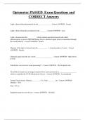
Simple Linear Regression Analysis
One independent variable X, and one dependent variable Y.
XY
Linear relationship means we can predict Y from X using a
'
linear function: Y =b 0+ b1 X
o Y ' = the predicted value of Y given X.
o b0 is the intercept; the predicted value Y ' when
someone scores 0 on X.
In practice often not very interesting.
o b1 is the regression coefficient; the change in Y ' when X increases with one unit – the
slope of the line.
o b0 and b1 are called parameters but b0 is not a predictor.
Simple regression analysis:
1. Find the best fitting straight line – find values for the coefficient (b0 and b1) – for
which we can best predict Y from X.
Line for which prediction errors are smallest (e i)
Choose b0 and b1 as such that e i is as small as possible.
This can be done by using ‘least squares estimation’:
N
∑ ¿¿
i=1
H0: b1 = 0 vs. H1: b1 ≠ 0
Least squares estimators for b0 and b1 can also be calculated from r XY and
the standard deviations (sx and sY).
sY
b 1=r
sX
X−X Y −Y
r =∑ ( Z ¿ ¿ X × ZY )÷ N , where Z X = ∧Z Y = ¿
SX SY
SPSS DOES THIS USUALLY.
Regression line always goes through the point where the averages intersect.
Estimated regression model:
, 2. Decide how well you can predict Y: inspect individual prediction errors.
e i ¿ Y i −Y 'i
e i is the prediction error for each person i (i = 1, i =2, …, N).
Difference between observed and predicted value Y.
The sum of the prediction errors will equal 0 – with a little deviation because
of rounding up or down.
Thus, the average prediction error is also 0.
Total variance = predicted variance + error variance:
s2Y =s2Y + s 2e
'
The variance of the prediction error is equal to the unexplained variance.
Process:
o Calculate 1-R2, which the proportion of unexplained
variance.
o To calculate total unexplained variance: proportion
2
unexplained variance times sY
R2 is the proportion explained by the variance.
1−R 2Y × X is the proportion of unexplained variance.
Ways to calculate R2
o
explained variance∈Y based ont h e regression SSregression
=
total variance∈Y SStotal
o With ONE predictor in model: R = absolute value of 𝛽1, so
squared 𝛽1 = R2
s 2Y '
o 2
s Y
3. Check whether you can generalize the results to the population level.
To answer this question, we use hypothesis tests:
H0: b1 = 0 – there is no linear association in the population.
H1: b1 ≠ 0 – there is a linear association in the population.
Test statistics:
b^ 1−b1
o t= : t-distribution, with df = N -2
SE ( b^ 1 )
o The SE( b^ ¿ ¿1) isthe standard error of b^ 1 ¿
o Note: df = N - #predictors -1 = dferrors’
Lecture 3
Interpretation of the Estimated Regression Coefficient b1
Y ' =b 0+ b1 X
First: two ways to interpret Y ' .
o Y ' = predicted Y given someone’s score on X.
o Y ' is an estimation of the average score on Y
for the population of people with a certain
value on X.
Interpretation regression coefficient b^ 1:
o When X increases with 1 unit, then Y ' increases with b^ 1 units.
Samples vs. Population
Types of Sampling Designs
Simple random sampling = every member in the population has an equal chance to be
sampled.
Stratified sampling = the population is divided into strata; within each stratum a random
sample is drawn.
Convenience sampling sample of people who are readily available.
Descriptive vs. Inferential Statistics
Descriptive statistics
o Summarizing data using measures of central tendency (mean, median, mode) or
measures of dispersion (variance, standard deviation).
Measures about central tendency and dispersion are only about one variable
(correlation is about two).
Inferential statistics = making generalization about the population.
o Procedures:
Null hypothesis significance testing
Steps:
1. Formulating H0 and H1.
2. Make a decision rule.
3. Obtain a t- and p-value from the output.
4. Either reject or keep H0 and draw a conclusion.
Reject if it is in critical regions or p-value < .05
Accept if it is in ‘normal’ region or p -value > .05
Confidence interval estimation
Definition: when we carry out an experiment over and over again,
the 95% CI will contain the real value of the parameter of interest in
95% of the cases.
Interpretation: based on the data, this would be the most probable
range of values for the real value of the correlation coefficient.
Importance: gives an indication of how precise the point estimate is.
Using CI for hypothesis testing: look whether the value of the
statistic under H0 (usually 0) lies within the interval.
o If it is, H0 will belong to the values from which we have 95%
certainty that it could possibly be the population value.
Level of Measurement
Classical measurement levels: nominal, ordinal, interval, ratio.
Categorial variable (e.g., gender).
Quantitative variable (e.g., IQ).
o More continuously measured.
Experimental, Quasi-Experimental, Correlational Studies
Correlational Studies
To measure the relationship between variables.
Pearson’s correlation coefficient.
o For measures of linear association between variables.
o Notation:
ρ = correlation in the population.
r = correlation in the sample.
, o -1 ≤ r ≤ 1
o r = 0: there is no linear association (but there might be non-linear association).
Statistical tests for the correlation coefficient:
o Inferential statistics:
1. H0: ρ = 0 vs. H1: ρ ≠ 0
T-test: t=r
√ N −2
1−r 2
with df = N – 2
SPSS gives the (two-sided) p-value for this test.
2. H0: ρ = c vs. H1: ρ ≠ c
C is a number between -1 and 1, but not 0.
Fisher Z-transformation and Z-tests are required (to test whether the
correlation in the sample is significantly larger than e.g., 0.8).
Not available in SPSS.
P-value = the p-value is the probability of the data in the sample (r) or more extreme (further
away from ), given that H0 (p = 0) is true.
o Use:
o Decide which significance level to use (usually 5% or 𝛼 = 0.05).
o When p < 𝛼, reject H0.
Lecture 2
Confidence Intervals for r:
CI ( 1−a) 100% =r ±Crit . Value(a ,two tailed ) × SE(r )
Crit. Value = the critical value depends on the desired confidence level.
SE(r) = the standard error.
o Describes variability in values of the sample (r) if you draw a large amount of samples
from the population.
CIs for correlation coefficients are not symmetric.
o Meaning r is usually not in the middle of the CI (due to Fisher transformations)).
Smaller N = wider interval – less precise.
Large sample = smaller CI – more precise measurements.
A 90% interval would be narrower than a 95% interval – gives more precise estimation.
Less certainty means more accuracy.
Assumptions for r:
Independence among observations.
o Is satisfied when a random sample has been drawn.
X and Y scores have a bivariate normal distribution.
o Scatterplot shaped like cigar.
X and Y are linearly related.
Assumption of homoscedasticity: scores on Y should (roughly) equal variance across levels of
X.
Power and Multiple Comparisons
Power = the probability to reject H0 given that H1 is true (there is really an effect).
Larger N smaller CI and more power.
To find small effects (p is small), a larger N is needed.
o Carry out power analysis before gathering data.
o N > 100 (to check assumptions, less impact of outliers).
When multiple comparisons are made (multiple correlations are tested), the probability of
making a Type I error (= incorrectly rejecting H0) will increase.
, o Replication
o Cross-validation.
o Bonferroni correction PC a =EW a /k
Squared Correlation
Another way to report effect size.
2
r XY = the proportion of the variance X you can linearly predict from Y – and vice versa.
o E.g., number of hours studying and exam grade correlate 0,40; thus 0.4 2 = 0.16
(16%) of difference in exam grades can be predicted by differences in the
number of hours studied.
Simple Linear Regression Analysis
One independent variable X, and one dependent variable Y.
XY
Linear relationship means we can predict Y from X using a
'
linear function: Y =b 0+ b1 X
o Y ' = the predicted value of Y given X.
o b0 is the intercept; the predicted value Y ' when
someone scores 0 on X.
In practice often not very interesting.
o b1 is the regression coefficient; the change in Y ' when X increases with one unit – the
slope of the line.
o b0 and b1 are called parameters but b0 is not a predictor.
Simple regression analysis:
1. Find the best fitting straight line – find values for the coefficient (b0 and b1) – for
which we can best predict Y from X.
Line for which prediction errors are smallest (e i)
Choose b0 and b1 as such that e i is as small as possible.
This can be done by using ‘least squares estimation’:
N
∑ ¿¿
i=1
H0: b1 = 0 vs. H1: b1 ≠ 0
Least squares estimators for b0 and b1 can also be calculated from r XY and
the standard deviations (sx and sY).
sY
b 1=r
sX
X−X Y −Y
r =∑ ( Z ¿ ¿ X × ZY )÷ N , where Z X = ∧Z Y = ¿
SX SY
SPSS DOES THIS USUALLY.
Regression line always goes through the point where the averages intersect.
Estimated regression model:
, 2. Decide how well you can predict Y: inspect individual prediction errors.
e i ¿ Y i −Y 'i
e i is the prediction error for each person i (i = 1, i =2, …, N).
Difference between observed and predicted value Y.
The sum of the prediction errors will equal 0 – with a little deviation because
of rounding up or down.
Thus, the average prediction error is also 0.
Total variance = predicted variance + error variance:
s2Y =s2Y + s 2e
'
The variance of the prediction error is equal to the unexplained variance.
Process:
o Calculate 1-R2, which the proportion of unexplained
variance.
o To calculate total unexplained variance: proportion
2
unexplained variance times sY
R2 is the proportion explained by the variance.
1−R 2Y × X is the proportion of unexplained variance.
Ways to calculate R2
o
explained variance∈Y based ont h e regression SSregression
=
total variance∈Y SStotal
o With ONE predictor in model: R = absolute value of 𝛽1, so
squared 𝛽1 = R2
s 2Y '
o 2
s Y
3. Check whether you can generalize the results to the population level.
To answer this question, we use hypothesis tests:
H0: b1 = 0 – there is no linear association in the population.
H1: b1 ≠ 0 – there is a linear association in the population.
Test statistics:
b^ 1−b1
o t= : t-distribution, with df = N -2
SE ( b^ 1 )
o The SE( b^ ¿ ¿1) isthe standard error of b^ 1 ¿
o Note: df = N - #predictors -1 = dferrors’
Lecture 3
Interpretation of the Estimated Regression Coefficient b1
Y ' =b 0+ b1 X
First: two ways to interpret Y ' .
o Y ' = predicted Y given someone’s score on X.
o Y ' is an estimation of the average score on Y
for the population of people with a certain
value on X.
Interpretation regression coefficient b^ 1:
o When X increases with 1 unit, then Y ' increases with b^ 1 units.