SOLUTIONS MANUAL Introduction to Probability and Statistics 15/E Mendenhall
1: Describing Data with Graphs
Section 1.1
1.1.1 The experimental unit, the individual or object on which a variable is measured, is the student.
1.1.2 The experimental unit on which the number of errors is measured is the exam.
1.1.3 The experimental unit is the patient.
1.1.4 The experimental unit is the azalea plant.
1.1.5 The experimental unit is the car.
1.1.6 “Time to assemble” is a quantitative variable because a numerical quantity (1 hour, 1.5 hours, etc.) is
measured.
1.1.7 “Number of students” is a quantitative variable because a numerical quantity (1, 2, etc.) is measured.
1.1.8 “Rating of a politician” is a qualitative variable since a quality (excellent, good, fair, poor) is measured.
1.1.9 “State of residence” is a qualitative variable since a quality (CA, MT, AL, etc.) is measured.
1.1.10 “Population” is a discrete variable because it can take on only integer values.
1.1.11 “Weight” is a continuous variable, taking on any values associated with an interval on the real line.
1.1.12 Number of claims is a discrete variable because it can take on only integer values.
1.1.13 “Number of consumers” is integer-valued and hence discrete.
1.1.14 “Number of boating accidents” is integer-valued and hence discrete.
1.1.15 “Time” is a continuous variable.
1.1.16 “Cost of a head of lettuce” is a discrete variable since money can be measured only in dollars and cents.
1.1.17 “Number of brothers and sisters” is integer-valued and hence discrete.
1.1.18 “Yield in bushels” is a continuous variable, taking on any values associated with an interval on the real
line.
1.1.19 The statewide database contains a record of all drivers in the state of Michigan. The data collected
represents the population of interest to the researcher.
1.1.20 The researcher is interested in the opinions of all citizens, not just the 1000 citizens that have been
interviewed. The responses of these 1000 citizens represent a sample.
1.1.21 The researcher is interested in the weight gain of all animals that might be put on this diet, not just the
twenty animals that have been observed. The responses of these twenty animals is a sample.
1.1.22 The data from the Internal Revenue Service contains the records of all wage earners in the United States.
The data collected represents the population of interest to the researcher.
1.1.23 a The experimental unit, the item or object on which variables are measured, is the vehicle.
b Type (qualitative); make (qualitative); carpool or not? (qualitative); one-way commute distance
(quantitative continuous); age of vehicle (quantitative continuous)
c Since five variables have been measured, this is multivariate data.
1.1.24 a The set of ages at death represents a population, because there have only been 38 different presidents
in the United States history.
b The variable being measured is the continuous variable “age”.
c “Age” is a quantitative variable.
1
,1.1.25 a The population of interest consists of voter opinions (for or against the candidate) at the time of the
election for all persons voting in the election.
b Note that when a sample is taken (at some time prior or the election), we are not actually sampling
from the population of interest. As time passes, voter opinions change. Hence, the population of voter
opinions changes with time, and the sample may not be representative of the population of interest.
1.1.26 a-b The variable “survival time” is a quantitative continuous variable.
c The population of interest is the population of survival times for all patients having a particular type
of cancer and having undergone a particular type of radiotherapy.
d-e Note that there is a problem with sampling in this situation. If we sample from all patients having
cancer and radiotherapy, some may still be living and their survival time will not be measurable. Hence,
we cannot sample directly from the population of interest, but must arrive at some reasonable alternate
population from which to sample.
1.1.27 a The variable “reading score” is a quantitative variable, which is probably integer-valued and hence
discrete.
b The individual on which the variable is measured is the student.
c The population is hypothetical – it does not exist in fact – but consists of the reading scores for all
students who could possibly be taught by this method.
Section 1.2
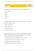
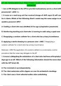
1.2.1 The pie chart is constructed by partitioning the circle into five parts, according to the total contributed by
each part. Since the total number of students is 100, the total number receiving a final grade of A
represents 31 100 = 0.31 or 31% of the total. Thus, this category will be represented by a sector angle of
0.31(360) = 111.6 . The other sector angles are shown next, along with the pie chart.
Final Grade Frequency Fraction of Total Sector Angle
A 31 .31 111.6
B 36 .36 129.6
C 21 .21 75.6
D 9 .09 32.4
F 3 .03 10.8
F
D 3.0%
9.0%
A
31.0%
C
21.0%
B
36.0%
2
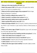
, The bar chart represents each category as a bar with height equal to the frequency of occurrence of that
category and is shown in the figure that follows.
40
30
Frequency
20
10
0
A B C D F
Final Grade
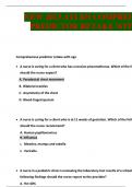
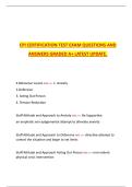
1.2.2 Construct a statistical table to summarize the data. The pie and bar charts are shown in the figures that
follow.
Status Frequency Fraction of Total Sector Angle
Freshman 32 .32 115.2
Sophomore 34 .34 122.4
Junior 17 .17 61.2
Senior 9 .09 32.4
Grad Student 8 .08 28.8
35
Grad Student
8.0%
30
Senior
9.0%
Freshman
32.0% 25
Frequency
20
Junior
17.0% 15
10
5
Sophomore 0
34.0% Freshman Sophomore Junior Senior Grad Student
Status
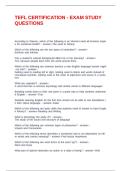
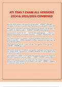
1.2.3 Construct a statistical table to summarize the data. The pie and bar charts are shown in the figures that
follow.
Status Frequency Fraction of Total Sector Angle
Humanities, Arts & Sciences 43 .43 154.8
Natural/Agricultural Sciences 32 .32 115.2
Business 17 .17 61.2
Other 8 .08 28.8
3
, other 40
8.0%
30
Frequency
Business
17.0%
20
Humanities, Arts & Sciences
43.0%
10
0
es es es
s
he
r
nc nc sin Ot
ie c ie
Sc lS Bu
s& r a
rt tu
,A ul
es ric
i ti Ag
Natural/Agricultural Sciences an al/
m u r
32.0% Hu at
N
College
1.2.4 a The pie chart is constructed by partitioning the circle into four parts, according to the total contributed
by each part. Since the total number of people is 50, the total number in category A represents
11 50 = 0.22 or 22% of the total. Thus, this category will be represented by a sector angle of
0.22(360) = 79.2o . The other sector angles are shown below. The pie chart is shown in the figure that
follows.
Category Frequency Fraction of Total Sector Angle
A 11 .22 79.2
B 14 .28 100.8
C 20 .40 144.0
D 5 .10 36.0
20
D
10.0%
A
22.0%
15
Frequency
10
C
40.0%
5
B
28.0%
0
A B C D
Category
b The bar chart represents each category as a bar with height equal to the frequency of occurrence of
that category and is shown in the figure above.
c Yes, the shape will change depending on the order of presentation. The order is unimportant.
d The proportion of people in categories B, C, or D is found by summing the frequencies in those three
categories, and dividing by n = 50. That is, (14 + 20 + 5) 50 = 0.78 .
e Since there are 14 people in category B, there are 50 −14 = 36 who are not, and the percentage is
calculated as ( 36 50 )100 = 72% .
1.2.5 a-b Construct a statistical table to summarize the data. The pie and bar charts are shown in the figures
that follow.
4
1: Describing Data with Graphs
Section 1.1
1.1.1 The experimental unit, the individual or object on which a variable is measured, is the student.
1.1.2 The experimental unit on which the number of errors is measured is the exam.
1.1.3 The experimental unit is the patient.
1.1.4 The experimental unit is the azalea plant.
1.1.5 The experimental unit is the car.
1.1.6 “Time to assemble” is a quantitative variable because a numerical quantity (1 hour, 1.5 hours, etc.) is
measured.
1.1.7 “Number of students” is a quantitative variable because a numerical quantity (1, 2, etc.) is measured.
1.1.8 “Rating of a politician” is a qualitative variable since a quality (excellent, good, fair, poor) is measured.
1.1.9 “State of residence” is a qualitative variable since a quality (CA, MT, AL, etc.) is measured.
1.1.10 “Population” is a discrete variable because it can take on only integer values.
1.1.11 “Weight” is a continuous variable, taking on any values associated with an interval on the real line.
1.1.12 Number of claims is a discrete variable because it can take on only integer values.
1.1.13 “Number of consumers” is integer-valued and hence discrete.
1.1.14 “Number of boating accidents” is integer-valued and hence discrete.
1.1.15 “Time” is a continuous variable.
1.1.16 “Cost of a head of lettuce” is a discrete variable since money can be measured only in dollars and cents.
1.1.17 “Number of brothers and sisters” is integer-valued and hence discrete.
1.1.18 “Yield in bushels” is a continuous variable, taking on any values associated with an interval on the real
line.
1.1.19 The statewide database contains a record of all drivers in the state of Michigan. The data collected
represents the population of interest to the researcher.
1.1.20 The researcher is interested in the opinions of all citizens, not just the 1000 citizens that have been
interviewed. The responses of these 1000 citizens represent a sample.
1.1.21 The researcher is interested in the weight gain of all animals that might be put on this diet, not just the
twenty animals that have been observed. The responses of these twenty animals is a sample.
1.1.22 The data from the Internal Revenue Service contains the records of all wage earners in the United States.
The data collected represents the population of interest to the researcher.
1.1.23 a The experimental unit, the item or object on which variables are measured, is the vehicle.
b Type (qualitative); make (qualitative); carpool or not? (qualitative); one-way commute distance
(quantitative continuous); age of vehicle (quantitative continuous)
c Since five variables have been measured, this is multivariate data.
1.1.24 a The set of ages at death represents a population, because there have only been 38 different presidents
in the United States history.
b The variable being measured is the continuous variable “age”.
c “Age” is a quantitative variable.
1
,1.1.25 a The population of interest consists of voter opinions (for or against the candidate) at the time of the
election for all persons voting in the election.
b Note that when a sample is taken (at some time prior or the election), we are not actually sampling
from the population of interest. As time passes, voter opinions change. Hence, the population of voter
opinions changes with time, and the sample may not be representative of the population of interest.
1.1.26 a-b The variable “survival time” is a quantitative continuous variable.
c The population of interest is the population of survival times for all patients having a particular type
of cancer and having undergone a particular type of radiotherapy.
d-e Note that there is a problem with sampling in this situation. If we sample from all patients having
cancer and radiotherapy, some may still be living and their survival time will not be measurable. Hence,
we cannot sample directly from the population of interest, but must arrive at some reasonable alternate
population from which to sample.
1.1.27 a The variable “reading score” is a quantitative variable, which is probably integer-valued and hence
discrete.
b The individual on which the variable is measured is the student.
c The population is hypothetical – it does not exist in fact – but consists of the reading scores for all
students who could possibly be taught by this method.
Section 1.2
1.2.1 The pie chart is constructed by partitioning the circle into five parts, according to the total contributed by
each part. Since the total number of students is 100, the total number receiving a final grade of A
represents 31 100 = 0.31 or 31% of the total. Thus, this category will be represented by a sector angle of
0.31(360) = 111.6 . The other sector angles are shown next, along with the pie chart.
Final Grade Frequency Fraction of Total Sector Angle
A 31 .31 111.6
B 36 .36 129.6
C 21 .21 75.6
D 9 .09 32.4
F 3 .03 10.8
F
D 3.0%
9.0%
A
31.0%
C
21.0%
B
36.0%
2
, The bar chart represents each category as a bar with height equal to the frequency of occurrence of that
category and is shown in the figure that follows.
40
30
Frequency
20
10
0
A B C D F
Final Grade
1.2.2 Construct a statistical table to summarize the data. The pie and bar charts are shown in the figures that
follow.
Status Frequency Fraction of Total Sector Angle
Freshman 32 .32 115.2
Sophomore 34 .34 122.4
Junior 17 .17 61.2
Senior 9 .09 32.4
Grad Student 8 .08 28.8
35
Grad Student
8.0%
30
Senior
9.0%
Freshman
32.0% 25
Frequency
20
Junior
17.0% 15
10
5
Sophomore 0
34.0% Freshman Sophomore Junior Senior Grad Student
Status
1.2.3 Construct a statistical table to summarize the data. The pie and bar charts are shown in the figures that
follow.
Status Frequency Fraction of Total Sector Angle
Humanities, Arts & Sciences 43 .43 154.8
Natural/Agricultural Sciences 32 .32 115.2
Business 17 .17 61.2
Other 8 .08 28.8
3
, other 40
8.0%
30
Frequency
Business
17.0%
20
Humanities, Arts & Sciences
43.0%
10
0
es es es
s
he
r
nc nc sin Ot
ie c ie
Sc lS Bu
s& r a
rt tu
,A ul
es ric
i ti Ag
Natural/Agricultural Sciences an al/
m u r
32.0% Hu at
N
College
1.2.4 a The pie chart is constructed by partitioning the circle into four parts, according to the total contributed
by each part. Since the total number of people is 50, the total number in category A represents
11 50 = 0.22 or 22% of the total. Thus, this category will be represented by a sector angle of
0.22(360) = 79.2o . The other sector angles are shown below. The pie chart is shown in the figure that
follows.
Category Frequency Fraction of Total Sector Angle
A 11 .22 79.2
B 14 .28 100.8
C 20 .40 144.0
D 5 .10 36.0
20
D
10.0%
A
22.0%
15
Frequency
10
C
40.0%
5
B
28.0%
0
A B C D
Category
b The bar chart represents each category as a bar with height equal to the frequency of occurrence of
that category and is shown in the figure above.
c Yes, the shape will change depending on the order of presentation. The order is unimportant.
d The proportion of people in categories B, C, or D is found by summing the frequencies in those three
categories, and dividing by n = 50. That is, (14 + 20 + 5) 50 = 0.78 .
e Since there are 14 people in category B, there are 50 −14 = 36 who are not, and the percentage is
calculated as ( 36 50 )100 = 72% .
1.2.5 a-b Construct a statistical table to summarize the data. The pie and bar charts are shown in the figures
that follow.
4