Summary MTS3
Week 1. Regression
Regression is about a simple linear model which calculates the outcome with the
correlaton coefcient (b or r) and the error.
A simple regression formula is: y = b0 + b1*X1 + e
- b0: the point where the line intersects the vertcal aais of the graph.
- b1: the slope of the line. A positve b1 describes a positve correlatonn where a
negatve b1 describes a negatve correlaton.
- X1: the predictve factor that afects the outcome y.
- E: the standard error for the partcipant (i).
More variables can be added in the formula as b2n b3 etc.
Y = (b0 + b1*X1 + b2*X2) + e
- Y: the outcome variable (DV).
- B1: the coefcient of the rrst predictor (X1) (IV).
- B2: the coefcient of the second predictor (X2) (IV).
With one predictve value we speak of a simple regressionn but when there are multple
predictve values we speak of multiple regression.
Predicting the model
Residues: the diferences between the predicted values and the observed values.
- Positve residue: when the observed values are greater than the predicted values.
- Negatve residue: when the observed values are smaller than the predicted values.
Sum of squared residue/residue sum of squares (SSy): to easily calculate with the
residualsn the residue values are squared and added together. This gives an idea of how
much ‘error’ there is in the model.
Goodness fi of ihe model: does the model rt with the observed data?
Sum squared diferences/ioial sum of squares (SSi): total amount between the base
model (predicted values) and the observed data. We can use the mean/average to to
answer the queston above.
Model sum of squares (SSm): the diference between SSt and SSy. When a beter rtng
model is added there is an improvement in the SSyn this can be compared by calculatng
SSm. When the SSm is very largen the regression model is very diferent from the
average. When the SSm is very smalln then the regression model is beter to use instead
of the average.
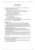
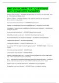
Figure 1. The rrst one (top lef) shows the SSTn which represents the diference between the
observed data and the average of the outcome Y.
The second graph (top right) shows the SSyn which represents the diference between
the observed data and the regression line.
The third graph (botom) shows the SSmn which represents the diference between
the average of Y and the regression line.
, R2 is the amount of variance in the outcome which is eaplained by the model (SSm)n
relatve to how much variance there was already in the rrst place (SSt). This can be
calculated by the formula: R2 = (SSm/SSt)
Mean squares of MS (MSm): the mean sum of squares; used to calculate the F-rato. This
can be calculated by the formula: F = (MSm/MSr)
F-ratio: calculates the diference between the predicted values and the observed values.
If the model is goodn we eapect great improvements in the predicted values where MSm
is large. With a small diference between the observed data and the modeln MSr is small.
A great model should have a large F-raton with a value larger than 1.
- To calculate the signircance from R2 we can use this formula:
F = ((N-k-1)R2) / (k(1-R2))
N is the number of partcipants; k is the number of variables in the model.
This F tests the null-hypothesis where R2 = 0.
Assessing individual predictve factors
Week 1. Regression
Regression is about a simple linear model which calculates the outcome with the
correlaton coefcient (b or r) and the error.
A simple regression formula is: y = b0 + b1*X1 + e
- b0: the point where the line intersects the vertcal aais of the graph.
- b1: the slope of the line. A positve b1 describes a positve correlatonn where a
negatve b1 describes a negatve correlaton.
- X1: the predictve factor that afects the outcome y.
- E: the standard error for the partcipant (i).
More variables can be added in the formula as b2n b3 etc.
Y = (b0 + b1*X1 + b2*X2) + e
- Y: the outcome variable (DV).
- B1: the coefcient of the rrst predictor (X1) (IV).
- B2: the coefcient of the second predictor (X2) (IV).
With one predictve value we speak of a simple regressionn but when there are multple
predictve values we speak of multiple regression.
Predicting the model
Residues: the diferences between the predicted values and the observed values.
- Positve residue: when the observed values are greater than the predicted values.
- Negatve residue: when the observed values are smaller than the predicted values.
Sum of squared residue/residue sum of squares (SSy): to easily calculate with the
residualsn the residue values are squared and added together. This gives an idea of how
much ‘error’ there is in the model.
Goodness fi of ihe model: does the model rt with the observed data?
Sum squared diferences/ioial sum of squares (SSi): total amount between the base
model (predicted values) and the observed data. We can use the mean/average to to
answer the queston above.
Model sum of squares (SSm): the diference between SSt and SSy. When a beter rtng
model is added there is an improvement in the SSyn this can be compared by calculatng
SSm. When the SSm is very largen the regression model is very diferent from the
average. When the SSm is very smalln then the regression model is beter to use instead
of the average.
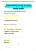
Figure 1. The rrst one (top lef) shows the SSTn which represents the diference between the
observed data and the average of the outcome Y.
The second graph (top right) shows the SSyn which represents the diference between
the observed data and the regression line.
The third graph (botom) shows the SSmn which represents the diference between
the average of Y and the regression line.
, R2 is the amount of variance in the outcome which is eaplained by the model (SSm)n
relatve to how much variance there was already in the rrst place (SSt). This can be
calculated by the formula: R2 = (SSm/SSt)
Mean squares of MS (MSm): the mean sum of squares; used to calculate the F-rato. This
can be calculated by the formula: F = (MSm/MSr)
F-ratio: calculates the diference between the predicted values and the observed values.
If the model is goodn we eapect great improvements in the predicted values where MSm
is large. With a small diference between the observed data and the modeln MSr is small.
A great model should have a large F-raton with a value larger than 1.
- To calculate the signircance from R2 we can use this formula:
F = ((N-k-1)R2) / (k(1-R2))
N is the number of partcipants; k is the number of variables in the model.
This F tests the null-hypothesis where R2 = 0.
Assessing individual predictve factors