Multiple Regression Analysis
• 1 DV (quantitative) = criterion
• 1 or more IV (quantitative) = predictors
Design:
• Criterion = name (quantitative)
• Predictor 1 = name (quantitative)
• Predictor 2 = name (quantitative)
Hypotheses:
• X = scores
• B = regression coefficients/weights
• (Ypredicted = B0 + B1*X1 + B2*X2 + ….)
• H0(general): β1 = β2 = …. = 0 (1,2 = predictors)
• H0(1name): β1 = 0
• H0(2name): β2 = 0
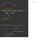
ANOVA table: general hypothesis tested
• Sources: regression, residual + total
• Df total = N-1
• Df regression = p
• Df residual = df total – df regression
• SS total = (N-1) * var(Y)
• SS regression = (N-1) * var(Ypredicted)
• SS residual = SS total – SS regression
• MS = SS / df
• F = MS regression/ MS residual
• R^2 = SS regression / SS total (this is the proportion explained variance)
• R = cor(Y,Ypred)
• R^2 > 0.20 strong
• R^2 between 0.10 and 0.20 medium
• R^2 < 0.10 weak
Decision:
In the prediction of the (DV) from the (IV’s), the R squared is/is not significantly larger than
0. Its value indicates a strong/medium/weak effect size. The regression coefficient of (IV1)
was significant/not significant. The regression coefficient of the (IV2) was significant/not
significant.
• Only indicate effect size if it is significantly larger
1
, Causal interpretation:
The variable (IV1) is experimental/not experimental, so in principle there is one/more than
one explanation for its predictive value as to (DV). The primary explanation is that …. An
alternative explanation is … (sometimes not obvious).
Extensions of multiple regression analysis
• Bi = standardized raw regression weights; changes if Y scores are multiplied by
constant c
o Can directly plug them into regression equation to predict new scores
• βi = standardized regression weights/beta weights; changes if Xi scores are multiplied
by constant c (only of that predictor, the beta weights of the other predictors remain
same)
o don’t depend on unit of measurement
• Bi = βi * S(Y)/s(Xi)
• B-weight: score Y 2x as large, B also 2x as large. Measurement 100x smaller, B also
100x smaller
• Beta-weight: Doesn’t change with measurement change.
(univariate) General Linear Model (GLM): Multiple regression analysis with dummy
codes for between-subject factors
Two-factor ANOVA: only for equal cell frequencies => regression: can deal with correlated
independent variables (unequal cell frequencies)
Short report:
A linear regression analysis with the … as dependent variable and the … and … as
independent variables, showed that the R squared is/ is not significantly larger than 0 F (df
regression, df residual) = F regression, p = p regression). Its value (R^2 = …) indicates a
strong/medium/weak effect size. The regression coefficient of the IV1 was significant/not
significant (beta = …, p = …). The regression coefficient of the IV2 was significant/not
significant (beta = …, p = …).
• Only indicate effect size if it is significant
GLM-Univariate
• 1 DV (quantitative) = criterion
• 1 or more IV = have to be between-subject factors
o Qualitative = between-subject factors
o Quantitative = covariates
Design:
• Dependent variable = name (quantitative)
• Between-subject factor = name (qualitative)
• Covariate 1 = name (quantitative)
2
• 1 DV (quantitative) = criterion
• 1 or more IV (quantitative) = predictors
Design:
• Criterion = name (quantitative)
• Predictor 1 = name (quantitative)
• Predictor 2 = name (quantitative)
Hypotheses:
• X = scores
• B = regression coefficients/weights
• (Ypredicted = B0 + B1*X1 + B2*X2 + ….)
• H0(general): β1 = β2 = …. = 0 (1,2 = predictors)
• H0(1name): β1 = 0
• H0(2name): β2 = 0
ANOVA table: general hypothesis tested
• Sources: regression, residual + total
• Df total = N-1
• Df regression = p
• Df residual = df total – df regression
• SS total = (N-1) * var(Y)
• SS regression = (N-1) * var(Ypredicted)
• SS residual = SS total – SS regression
• MS = SS / df
• F = MS regression/ MS residual
• R^2 = SS regression / SS total (this is the proportion explained variance)
• R = cor(Y,Ypred)
• R^2 > 0.20 strong
• R^2 between 0.10 and 0.20 medium
• R^2 < 0.10 weak
Decision:
In the prediction of the (DV) from the (IV’s), the R squared is/is not significantly larger than
0. Its value indicates a strong/medium/weak effect size. The regression coefficient of (IV1)
was significant/not significant. The regression coefficient of the (IV2) was significant/not
significant.
• Only indicate effect size if it is significantly larger
1
, Causal interpretation:
The variable (IV1) is experimental/not experimental, so in principle there is one/more than
one explanation for its predictive value as to (DV). The primary explanation is that …. An
alternative explanation is … (sometimes not obvious).
Extensions of multiple regression analysis
• Bi = standardized raw regression weights; changes if Y scores are multiplied by
constant c
o Can directly plug them into regression equation to predict new scores
• βi = standardized regression weights/beta weights; changes if Xi scores are multiplied
by constant c (only of that predictor, the beta weights of the other predictors remain
same)
o don’t depend on unit of measurement
• Bi = βi * S(Y)/s(Xi)
• B-weight: score Y 2x as large, B also 2x as large. Measurement 100x smaller, B also
100x smaller
• Beta-weight: Doesn’t change with measurement change.
(univariate) General Linear Model (GLM): Multiple regression analysis with dummy
codes for between-subject factors
Two-factor ANOVA: only for equal cell frequencies => regression: can deal with correlated
independent variables (unequal cell frequencies)
Short report:
A linear regression analysis with the … as dependent variable and the … and … as
independent variables, showed that the R squared is/ is not significantly larger than 0 F (df
regression, df residual) = F regression, p = p regression). Its value (R^2 = …) indicates a
strong/medium/weak effect size. The regression coefficient of the IV1 was significant/not
significant (beta = …, p = …). The regression coefficient of the IV2 was significant/not
significant (beta = …, p = …).
• Only indicate effect size if it is significant
GLM-Univariate
• 1 DV (quantitative) = criterion
• 1 or more IV = have to be between-subject factors
o Qualitative = between-subject factors
o Quantitative = covariates
Design:
• Dependent variable = name (quantitative)
• Between-subject factor = name (qualitative)
• Covariate 1 = name (quantitative)
2