4.4C: Applied Multivariate Data Analysis
Lecture 1: Field Chapter 2
Statistical Models
• Models → parameters + variables
• Parameters are estimated from the data and represent constant relations between
variables in the model
- Compute model parameters in the sample to estimate the value in the population
• e.g. linear regression → slope and intercept are the parameters
Model Fit
• Mean is a model of what happens in the real world: the typical score
- Not a perfect representation of the data
Calculating the Error
• The mean is the value from which the (squared) scores deviate the least (least error)
• Sum of squared errors, mean squared error/variance, standard deviation →
summarise how well the mean represents the sample data
• Sum of squared errors (sum of squares [SS]):
,Mean Squared Error
• Total dispersion depends on sample size → more informative to compute average
dispersion
- Mean of the squared errors (MSE) → closer to the mean is a better fit
- The larger the SS than MSE, the worse the fit
• ‘Average’ by dividing by the degrees of freedom (N – 1)
- Because sample data is used to estimate the model fit in the population
• Less overlap of confidence intervals = bigger difference
- If overlap more than half then means are not significantly different
Mean as a Model: Variance as Simple Measure of Model Fit
• General principle of model fit: sum (SSE) or average (MSE) the squared
deviations from the model
- Larger values indicate a lack of fit
• When the model is the mean, the MSE is called variance
- Mean squared error is the same as variance
• The square root of variance (s2) is called the standard deviation (s)
- Average deviation from the mean, not in squared units but in the original units
Standard Deviation and Shape of a Sample Distribution
, • Normal distribution occurs in nature → if you have many independent units of
information
• t-value that is about 2 → will be almost significant
• t-value that is about 3 or 4 → will be very significant
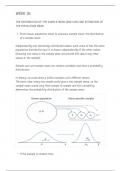
From Sample to Population
• Mean (X̄) and SD (s) are obtained from a sample, but used to estimate the mean (µ)
and SD (σ) of the population
• Sampling distribution → how the parameter of interest differs across the repeated
process of sampling from the distribution (distribution of sample means)
- Average discrepancy between the means estimated from the samples is the
variability of the sampling distribution
➔ It will have a width but as you go higher, the more infrequent that value will
get because more likely to be in middle of the distribution
▪ p-value is based on this
• One sample will provide an estimate of the true population parameter
- Depending on the variability AND sample size this estimate will be more or less
precise
• SD of the means of all possible samples of size N from the population → Standard
Error (SE) of the mean
Standard Error of the Mean
• Central limit theorem → for sample size ≥ 30, the sampling distribution of sample
means is a normal distribution with mean µσ and standard deviation σX̄
• σX̄ estimated from the sample by:
- s = sample SD
- SE → on average how much sample mean will differ from population mean
• The larger N:
- The smaller SE
- The more the sample mean is representative of the population mean (the more
precise the estimate)
• Can use the SE to calculate boundaries within is believed the population mean will lie
, Standard Error and Confidence Intervals
• 95% CI: for 95% of all possible samples the population mean will be within its limits
- In 5% of cases the estimate will be wrong
- 95% of data = 2 standard deviations above and below the mean
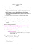
• 95% CI calculated by assuming the t-distribution as representative of the sampling
distribution
- t-distribution looks like the standard normal distribution, but fatter tails depending
on the df
• Lower limit of CI → X̄ − (𝑡𝑛−1 × SE)
• Upper limit of CI → X̄ + (𝑡𝑛−1 × SE)
- n – 1 are the degrees of freedom
- 𝑡𝑛−1 × SE is called the margin of error
Reporting and Interpreting CIs
• 95% corresponds to α = .05
- 90% and 99% CIs can also be used
• APA: M = 8.0; 95% CI [6.0, 10.0]
Lecture 1: Field Chapter 2
Statistical Models
• Models → parameters + variables
• Parameters are estimated from the data and represent constant relations between
variables in the model
- Compute model parameters in the sample to estimate the value in the population
• e.g. linear regression → slope and intercept are the parameters
Model Fit
• Mean is a model of what happens in the real world: the typical score
- Not a perfect representation of the data
Calculating the Error
• The mean is the value from which the (squared) scores deviate the least (least error)
• Sum of squared errors, mean squared error/variance, standard deviation →
summarise how well the mean represents the sample data
• Sum of squared errors (sum of squares [SS]):
,Mean Squared Error
• Total dispersion depends on sample size → more informative to compute average
dispersion
- Mean of the squared errors (MSE) → closer to the mean is a better fit
- The larger the SS than MSE, the worse the fit
• ‘Average’ by dividing by the degrees of freedom (N – 1)
- Because sample data is used to estimate the model fit in the population
• Less overlap of confidence intervals = bigger difference
- If overlap more than half then means are not significantly different
Mean as a Model: Variance as Simple Measure of Model Fit
• General principle of model fit: sum (SSE) or average (MSE) the squared
deviations from the model
- Larger values indicate a lack of fit
• When the model is the mean, the MSE is called variance
- Mean squared error is the same as variance
• The square root of variance (s2) is called the standard deviation (s)
- Average deviation from the mean, not in squared units but in the original units
Standard Deviation and Shape of a Sample Distribution
, • Normal distribution occurs in nature → if you have many independent units of
information
• t-value that is about 2 → will be almost significant
• t-value that is about 3 or 4 → will be very significant
From Sample to Population
• Mean (X̄) and SD (s) are obtained from a sample, but used to estimate the mean (µ)
and SD (σ) of the population
• Sampling distribution → how the parameter of interest differs across the repeated
process of sampling from the distribution (distribution of sample means)
- Average discrepancy between the means estimated from the samples is the
variability of the sampling distribution
➔ It will have a width but as you go higher, the more infrequent that value will
get because more likely to be in middle of the distribution
▪ p-value is based on this
• One sample will provide an estimate of the true population parameter
- Depending on the variability AND sample size this estimate will be more or less
precise
• SD of the means of all possible samples of size N from the population → Standard
Error (SE) of the mean
Standard Error of the Mean
• Central limit theorem → for sample size ≥ 30, the sampling distribution of sample
means is a normal distribution with mean µσ and standard deviation σX̄
• σX̄ estimated from the sample by:
- s = sample SD
- SE → on average how much sample mean will differ from population mean
• The larger N:
- The smaller SE
- The more the sample mean is representative of the population mean (the more
precise the estimate)
• Can use the SE to calculate boundaries within is believed the population mean will lie
, Standard Error and Confidence Intervals
• 95% CI: for 95% of all possible samples the population mean will be within its limits
- In 5% of cases the estimate will be wrong
- 95% of data = 2 standard deviations above and below the mean
• 95% CI calculated by assuming the t-distribution as representative of the sampling
distribution
- t-distribution looks like the standard normal distribution, but fatter tails depending
on the df
• Lower limit of CI → X̄ − (𝑡𝑛−1 × SE)
• Upper limit of CI → X̄ + (𝑡𝑛−1 × SE)
- n – 1 are the degrees of freedom
- 𝑡𝑛−1 × SE is called the margin of error
Reporting and Interpreting CIs
• 95% corresponds to α = .05
- 90% and 99% CIs can also be used
• APA: M = 8.0; 95% CI [6.0, 10.0]