SMCR – NOTES CHAPTER 1 – 11
CHAPTER 1
The characteristics of the samples that we could have drawn constitute a sampling
distribution.
Simulation = we let a computer draw many random samples from a population
1.1 Statistical Inference
Inferential statistics offers techniques for making statements about a larger set of
observations from data collected for a smaller set of observations. The large set of
observations about which we want to make a statement is called the population. The
smaller set is called a sample.
We want to generalize a statement about the sample to a statement about the
population from which the sample was drawn.
1.2 A discrete random variable
1.2.1 Sample statistic
The number of yellow candies in a bag (=sample) is an example of sample statistic:
a value describing a characteristic of the sample (in this case-> number of yellow
candies in a bag)
The collection of all possible outcome scores is called the sampling space (->
numbers 0 to 10)
The sample statistic is called a random variable. It is a variable because different
samples can vary and have different scores. Random because the score depends on
chance.
1.2.2 Sampling distribution
We call the distribution of the outcome scores of very many samples a sampling
distribution
,1.2.3 Probability and probability distribution
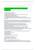
The probability is the proportion of all possible samples that we could have drawn
that happen to contain a specific n of yellow candies. It depends on the share of
yellow candies in the population of all candies
The figure shows a discrete probability distribution cause only a limited number of
outcomes are possible
To calculate the probability that we get a sample with five yellow candies -> divide
the number of samples with five y candies by the total number of samples that
have been drawn.
Probability distribution of the sample statistic = if we change the frequencies in
the sampling distribution into proportions/probabilities
-> a sampling space with a probability between 0 and 1 for each outcome of the
sample statistic
Probability distribution tells us
1. What the expected outcome can be
2. The probability that a particular outcome may occur
,1.2.4 Expected value or expectation
The expected value of the proportion of yellow candies in the sample is equal to the
proportion of yellow candies in the population.
Definition = the expected value (also called expectation) is the average (mean) of the
sampling distribution of a random variable
1.2.5 Unbiased estimator - representativeness. Sample is representative of the
population
The sample statistic equals the population statistic, for this reason the sample
proportion is an unbiased estimator of the proportion in the population.
Generally -> a sample statistic is called an unbiased estimator of the population
statistic if the expected value (mean of the sampling distribution) is equal to the
population statistic (/parameter)
If we take the parameter as estimator of the sample statistic, this estimate will be
downward biased = too low.
we must calculate the standard deviation and variance in the sample in a special
way to obtain an unbiased estimate of the population standard deviation and
variance.
1.2.6 Representative sample
A sample is representative of a population (in the strict sense) if variables in the
sample are distributed in the same way as in the population.
we should expect it to be representative, so we say that it is in principle
representative or representative in the statistical sense of the population. We
can use probability theory to account for the misrepresentation in the actual sample
that we draw.
1.3 A continuous Random Variable: overweight and underweight
, A variable is continuous if we can always think of a new value in between two values
1.3.2 Continuous sample statistic
The average weight of candies in our sample bag is our key sample statistic
Probabilities that we get (for example) an average candy weight of exactly 2.8 grams
are virtually 0.
1.3.3 Probability density
With a continuous sample statistic, we must look at a range of values instead of a
single value. The probability of getting an average weight of 2 is between 0 and
nearly 0 (range!!!)
• We choose a threshold (e.g. 2.8g)
• Determine the probability of values above or below this threshold
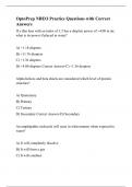
How can we display probabilities?
We have to display a probability as an area between the horizontal axis and a curve.
This curve = a probability density function
Vertical axis of the continuous probability distribution = "probability density"
• Left-hand probability = the probability of values up to (and including) a
threshold value. If it includes the left-hand tail
• Right-hand probability = the probability of values above (and including) a
threshold value. If it includes the right-hand tail
In a null hypothesis testing, these two are used to calculate p values
1.3.4 Probabilities always sum to 1
Displayed probabilities always add up to one.
1.4 Concluding Remarks
1.4.1 Sample characteristics as observations
CHAPTER 1
The characteristics of the samples that we could have drawn constitute a sampling
distribution.
Simulation = we let a computer draw many random samples from a population
1.1 Statistical Inference
Inferential statistics offers techniques for making statements about a larger set of
observations from data collected for a smaller set of observations. The large set of
observations about which we want to make a statement is called the population. The
smaller set is called a sample.
We want to generalize a statement about the sample to a statement about the
population from which the sample was drawn.
1.2 A discrete random variable
1.2.1 Sample statistic
The number of yellow candies in a bag (=sample) is an example of sample statistic:
a value describing a characteristic of the sample (in this case-> number of yellow
candies in a bag)
The collection of all possible outcome scores is called the sampling space (->
numbers 0 to 10)
The sample statistic is called a random variable. It is a variable because different
samples can vary and have different scores. Random because the score depends on
chance.
1.2.2 Sampling distribution
We call the distribution of the outcome scores of very many samples a sampling
distribution
,1.2.3 Probability and probability distribution
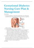
The probability is the proportion of all possible samples that we could have drawn
that happen to contain a specific n of yellow candies. It depends on the share of
yellow candies in the population of all candies
The figure shows a discrete probability distribution cause only a limited number of
outcomes are possible
To calculate the probability that we get a sample with five yellow candies -> divide
the number of samples with five y candies by the total number of samples that
have been drawn.
Probability distribution of the sample statistic = if we change the frequencies in
the sampling distribution into proportions/probabilities
-> a sampling space with a probability between 0 and 1 for each outcome of the
sample statistic
Probability distribution tells us
1. What the expected outcome can be
2. The probability that a particular outcome may occur
,1.2.4 Expected value or expectation
The expected value of the proportion of yellow candies in the sample is equal to the
proportion of yellow candies in the population.
Definition = the expected value (also called expectation) is the average (mean) of the
sampling distribution of a random variable
1.2.5 Unbiased estimator - representativeness. Sample is representative of the
population
The sample statistic equals the population statistic, for this reason the sample
proportion is an unbiased estimator of the proportion in the population.
Generally -> a sample statistic is called an unbiased estimator of the population
statistic if the expected value (mean of the sampling distribution) is equal to the
population statistic (/parameter)
If we take the parameter as estimator of the sample statistic, this estimate will be
downward biased = too low.
we must calculate the standard deviation and variance in the sample in a special
way to obtain an unbiased estimate of the population standard deviation and
variance.
1.2.6 Representative sample
A sample is representative of a population (in the strict sense) if variables in the
sample are distributed in the same way as in the population.
we should expect it to be representative, so we say that it is in principle
representative or representative in the statistical sense of the population. We
can use probability theory to account for the misrepresentation in the actual sample
that we draw.
1.3 A continuous Random Variable: overweight and underweight
, A variable is continuous if we can always think of a new value in between two values
1.3.2 Continuous sample statistic
The average weight of candies in our sample bag is our key sample statistic
Probabilities that we get (for example) an average candy weight of exactly 2.8 grams
are virtually 0.
1.3.3 Probability density
With a continuous sample statistic, we must look at a range of values instead of a
single value. The probability of getting an average weight of 2 is between 0 and
nearly 0 (range!!!)
• We choose a threshold (e.g. 2.8g)
• Determine the probability of values above or below this threshold
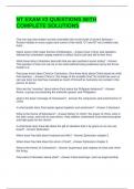
How can we display probabilities?
We have to display a probability as an area between the horizontal axis and a curve.
This curve = a probability density function
Vertical axis of the continuous probability distribution = "probability density"
• Left-hand probability = the probability of values up to (and including) a
threshold value. If it includes the left-hand tail
• Right-hand probability = the probability of values above (and including) a
threshold value. If it includes the right-hand tail
In a null hypothesis testing, these two are used to calculate p values
1.3.4 Probabilities always sum to 1
Displayed probabilities always add up to one.
1.4 Concluding Remarks
1.4.1 Sample characteristics as observations