Statistics 2.0
Exam: Wednesday 27 t h of March, 2019
INDEX
1. Rehearsing Statistics 1 2
® The basis 2
® Testing 6
2. Relations between two, three and more variables 8
® Simple linear regression 8
® Multivariate relations 11
3. Multiple regression 13
4. Analysis of variance with 1 factor 19
® ANOVA 1: Testing hypotheses & confidence intervals 19
® ANOVA 2: Effect sizes, dummy regression model & repeated measures ANOVA 23
5. Analysis of variance with more factors; analysis of covariance 26
® Two-way ANOVA: Analysis of variance with two factors 26
® ANCOVA: Analysis of variance with one factor and one covariate 32
6. Modelbuliding and assumptions 35
7. The Generalized Linear Model 40
8. Mentimeter Quiz 42
This summary includes (almost) everything from the lectures & the book for the Statistics II material. The
materials for Statistics I (chapter 1) only consists of the material discussed in the lecture.
CLAIMER
This summary is made by a student!
Studying from it and relying on it for 100% is your own responsibility.
THANKS & GOOD LUCK!!! J
J YOU CAN DO IT !!!!
, 2
Rehearsing Statistics 1 (Agresti, Ch. 1 – 8)
THE BASIS
Variables and their Measurement levels
- Variable – a characteristics that can vary in value among subjects in a sample or population (e.g.
XTC use)
o Variables each have their own measurement level
o Variable can take different “forms” (e.g. for XTC use: yes/no)
- Measurement level determines statistical technique to be used
- 4 different levels
o Nominal – at most classification in unordered categories
§ Does this category apply to this observation or not? Coding can be done with
numbers, letters, or symbols
o Ordinal – at most classification in ordered categories
§ Classification as ‘larger than’, ‘equal to’ or ‘smaller than’
§ Rank ordering: from high to low, from low to high
§ Nominal and ordinal together are categorical
§ We cannot interpret the difference in scores
§ Ordinal variables are ‘fuzzy’ – e.g. sum score of Likert scales
o Interval – besides ordering differences are interpretable as equal measurement units
o Ratio – besides ordering and equal measurement units there is absolute zero point
§ Interval and ratio together are metric or quantitative
- Measurement levels in practice
o Most methods suitable for interval and ratio (‘parametric methods’)
§ Nonparametric are less known and less used
o In practice, parametric methods are often used for ordinal and discrete data with many
possible values (e.g. Likert scales with 7 values or more – discrete à continuous)
Descriptive statistics
- Descriptive statistics are about summarizing data with tables and figures
o NO testing, no conclusions
o Can describe one variable or associations between multiple variables
o Different for categorical and quantitative data
o ALWAYS explore data before actually analyzing them!!!
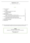
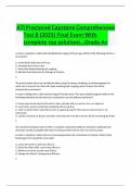
- CATEGORICAL
o E.g. an exam question with 4
answers.
o Categorical variable (nominal)
o The frequency table describes the
frequencies per category
§ Can also determine proportion & percentage
o For each answer you can also make a figure: plot the frequency and the answer – bar graph
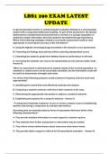
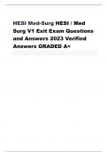
- QUANTITATIVE
o E.g. data on how many correct answers ppl
had on an exam (0 – 24)
o Frequency table now uses intervals for the
many values of this quantitative variable (e.g.
in this case they used steps of 2)
o Can also make figure - histogram
§ Use the intervals of quantitative scores
, 3
§ Bars are CONNECTED because the scale is quantitative (quite normally distributed as
well)
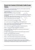
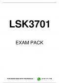
o Stem and leaf-plot
§ Actually histogram but turned to the side
§ How to read?
• 0 row: just numbers like 8 and 9
• 1 row: these are “in the tens”, so e.g. a
3 in that row means 13. Just like that a 3 in the “2 row” means 23.
• Each number is a subject!
§ More informative than a histogram because it also shows
the frequency with which a specific number has appeared
(e.g. 4 people scored 15)
- Description of forms of distribution
o Normal distribution – bell shaped – clock form
§ Many variables are normally distributed
o Also other forms!
§ U-shaped
• Not very often in psychology,
sometimes when researching
attitudes (e.g. opinion on abortion)
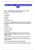
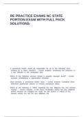
§ Skewed distributions
• LEFT graph = skewed to left =
negative skew (many people
score higher)
• RIGHT graph = skewed to right
= positive skew (many people
score lower)
• Have to know where the
mean/median/mode is in skewed distribution!!!
- Description of data variability! (mean does not tell us everything)
o Range – difference between max and min
o Deviation – how much does a certain value differ
from the mean. Deviation 𝑦( − 𝑦"
o Sum of squares – calculate the differences for each Sum of squares ∑(𝑦( − 𝑦"),
value with the mean, square this difference and add ∑(./ 0.")1
them all up Variance 𝑠 , = 203
o Variance – measure of spread in the data
o Standard deviation – measure of spread in the data ∑(./ 0.")1
Standard deviation 𝑠 = 4 203
- The empirical rule – normal distribution
o If data is normally distributed (resembles a
clock form):
§ About 68% of the observations lie
within a distance of one standard
deviation from the mean (between 𝑦" −
𝑠 and 𝑦" + 𝑠)
§ About 95% of the observations lie
within a distance of two standard
deviations from the mean (between
𝑦" − 2𝑠 and 𝑦" + 2𝑠)
§ Almost all observations lie within 3 standard deviations from the mean (between
𝑦" − 3𝑠 and 𝑦" + 3𝑠)
, 4
- Measures of position
o Quartiles – divide data up in four equal parts
o Interquartile range (IQR) – difference between first and third quartile
o Outlier – a score that is very extreme. You can
classify a score as an outlier as follows: if the
score is (1.5 * IQR) above or below the 3rd or 1st
quartile, it is an outlier.
§ Example: your score is -3, the 1st
quartile is 4, the 3rd quartile is 8, so the
IQR = 4.
§ 1.5 * 4 = 6
§ Below 1st quartile: 4 – 6 = -2 à your score classifies as an outlier because -3 is
further away from the 1st quartile than -2.
Probability distributions
- Probability – the chance than an observation takes on a particular value
- Probability distribution – all possible values of a variable and their probabilities
o Discrete probability distributions: each possible value has a probability, histogram with on
the y-axis the probabilities
o Continuous probability distributions: infinite number of possible values, probabilities of
chosen intervals of values. Figure with probability = area under the curve
- Population distribution
o Shows how the trait is actually distributed in the population.
o Can use values that result from this distribution (e.g. mean, sd) to determine the probability
on a certain score on y.
.0 7
o Use 𝑧 = 8
§ Fill in the sd, mean and y-score, then search for the probability in the z-table
o The population distribution uses parameters (often unknown, can be estimated)
- Sample distribution
o Shows how the trait is distributed in the sample
o Use sample statistics
o Larger the sample the better
- Sampling distribution
o Distribution of sample statistic (sample means) across samples
o Mean of the sampling distribution of 𝑦" is µ.
8
o The standard deviation of the sampling distribution of 𝑦" is the standard error 𝜎." =
√2
o The sampling distribution shows less spread than the population distribution, because:
§ Extreme values have a smaller probability to be drawn than central values
§ Drawing many extreme values is even less likely
§ These extreme values should then be extreme on one side
§ Extreme values are usually compensated by central values or an extreme value on
the other
side
Exam: Wednesday 27 t h of March, 2019
INDEX
1. Rehearsing Statistics 1 2
® The basis 2
® Testing 6
2. Relations between two, three and more variables 8
® Simple linear regression 8
® Multivariate relations 11
3. Multiple regression 13
4. Analysis of variance with 1 factor 19
® ANOVA 1: Testing hypotheses & confidence intervals 19
® ANOVA 2: Effect sizes, dummy regression model & repeated measures ANOVA 23
5. Analysis of variance with more factors; analysis of covariance 26
® Two-way ANOVA: Analysis of variance with two factors 26
® ANCOVA: Analysis of variance with one factor and one covariate 32
6. Modelbuliding and assumptions 35
7. The Generalized Linear Model 40
8. Mentimeter Quiz 42
This summary includes (almost) everything from the lectures & the book for the Statistics II material. The
materials for Statistics I (chapter 1) only consists of the material discussed in the lecture.
CLAIMER
This summary is made by a student!
Studying from it and relying on it for 100% is your own responsibility.
THANKS & GOOD LUCK!!! J
J YOU CAN DO IT !!!!
, 2
Rehearsing Statistics 1 (Agresti, Ch. 1 – 8)
THE BASIS
Variables and their Measurement levels
- Variable – a characteristics that can vary in value among subjects in a sample or population (e.g.
XTC use)
o Variables each have their own measurement level
o Variable can take different “forms” (e.g. for XTC use: yes/no)
- Measurement level determines statistical technique to be used
- 4 different levels
o Nominal – at most classification in unordered categories
§ Does this category apply to this observation or not? Coding can be done with
numbers, letters, or symbols
o Ordinal – at most classification in ordered categories
§ Classification as ‘larger than’, ‘equal to’ or ‘smaller than’
§ Rank ordering: from high to low, from low to high
§ Nominal and ordinal together are categorical
§ We cannot interpret the difference in scores
§ Ordinal variables are ‘fuzzy’ – e.g. sum score of Likert scales
o Interval – besides ordering differences are interpretable as equal measurement units
o Ratio – besides ordering and equal measurement units there is absolute zero point
§ Interval and ratio together are metric or quantitative
- Measurement levels in practice
o Most methods suitable for interval and ratio (‘parametric methods’)
§ Nonparametric are less known and less used
o In practice, parametric methods are often used for ordinal and discrete data with many
possible values (e.g. Likert scales with 7 values or more – discrete à continuous)
Descriptive statistics
- Descriptive statistics are about summarizing data with tables and figures
o NO testing, no conclusions
o Can describe one variable or associations between multiple variables
o Different for categorical and quantitative data
o ALWAYS explore data before actually analyzing them!!!
- CATEGORICAL
o E.g. an exam question with 4
answers.
o Categorical variable (nominal)
o The frequency table describes the
frequencies per category
§ Can also determine proportion & percentage
o For each answer you can also make a figure: plot the frequency and the answer – bar graph
- QUANTITATIVE
o E.g. data on how many correct answers ppl
had on an exam (0 – 24)
o Frequency table now uses intervals for the
many values of this quantitative variable (e.g.
in this case they used steps of 2)
o Can also make figure - histogram
§ Use the intervals of quantitative scores
, 3
§ Bars are CONNECTED because the scale is quantitative (quite normally distributed as
well)
o Stem and leaf-plot
§ Actually histogram but turned to the side
§ How to read?
• 0 row: just numbers like 8 and 9
• 1 row: these are “in the tens”, so e.g. a
3 in that row means 13. Just like that a 3 in the “2 row” means 23.
• Each number is a subject!
§ More informative than a histogram because it also shows
the frequency with which a specific number has appeared
(e.g. 4 people scored 15)
- Description of forms of distribution
o Normal distribution – bell shaped – clock form
§ Many variables are normally distributed
o Also other forms!
§ U-shaped
• Not very often in psychology,
sometimes when researching
attitudes (e.g. opinion on abortion)
§ Skewed distributions
• LEFT graph = skewed to left =
negative skew (many people
score higher)
• RIGHT graph = skewed to right
= positive skew (many people
score lower)
• Have to know where the
mean/median/mode is in skewed distribution!!!
- Description of data variability! (mean does not tell us everything)
o Range – difference between max and min
o Deviation – how much does a certain value differ
from the mean. Deviation 𝑦( − 𝑦"
o Sum of squares – calculate the differences for each Sum of squares ∑(𝑦( − 𝑦"),
value with the mean, square this difference and add ∑(./ 0.")1
them all up Variance 𝑠 , = 203
o Variance – measure of spread in the data
o Standard deviation – measure of spread in the data ∑(./ 0.")1
Standard deviation 𝑠 = 4 203
- The empirical rule – normal distribution
o If data is normally distributed (resembles a
clock form):
§ About 68% of the observations lie
within a distance of one standard
deviation from the mean (between 𝑦" −
𝑠 and 𝑦" + 𝑠)
§ About 95% of the observations lie
within a distance of two standard
deviations from the mean (between
𝑦" − 2𝑠 and 𝑦" + 2𝑠)
§ Almost all observations lie within 3 standard deviations from the mean (between
𝑦" − 3𝑠 and 𝑦" + 3𝑠)
, 4
- Measures of position
o Quartiles – divide data up in four equal parts
o Interquartile range (IQR) – difference between first and third quartile
o Outlier – a score that is very extreme. You can
classify a score as an outlier as follows: if the
score is (1.5 * IQR) above or below the 3rd or 1st
quartile, it is an outlier.
§ Example: your score is -3, the 1st
quartile is 4, the 3rd quartile is 8, so the
IQR = 4.
§ 1.5 * 4 = 6
§ Below 1st quartile: 4 – 6 = -2 à your score classifies as an outlier because -3 is
further away from the 1st quartile than -2.
Probability distributions
- Probability – the chance than an observation takes on a particular value
- Probability distribution – all possible values of a variable and their probabilities
o Discrete probability distributions: each possible value has a probability, histogram with on
the y-axis the probabilities
o Continuous probability distributions: infinite number of possible values, probabilities of
chosen intervals of values. Figure with probability = area under the curve
- Population distribution
o Shows how the trait is actually distributed in the population.
o Can use values that result from this distribution (e.g. mean, sd) to determine the probability
on a certain score on y.
.0 7
o Use 𝑧 = 8
§ Fill in the sd, mean and y-score, then search for the probability in the z-table
o The population distribution uses parameters (often unknown, can be estimated)
- Sample distribution
o Shows how the trait is distributed in the sample
o Use sample statistics
o Larger the sample the better
- Sampling distribution
o Distribution of sample statistic (sample means) across samples
o Mean of the sampling distribution of 𝑦" is µ.
8
o The standard deviation of the sampling distribution of 𝑦" is the standard error 𝜎." =
√2
o The sampling distribution shows less spread than the population distribution, because:
§ Extreme values have a smaller probability to be drawn than central values
§ Drawing many extreme values is even less likely
§ These extreme values should then be extreme on one side
§ Extreme values are usually compensated by central values or an extreme value on
the other
side