Week 1: Data types, describing and exploring your data
The type of statistical analysis depends on the type of variable
QUALITATIVE variable: outcomes are categories
4. Nominal: unordered categories (Male/Female)
3. Categorical: ordered categories (Likert scale, Job skill)
QUANTITATIVE variables: outcomes are numbers
2. Discrete: series of isolated numbers (numbers of cars sold, change in
employees)
1. Continuous: interval of possible values (BNP, temperature)
A variable can always be treated as a lower type.
For QUALITATIVE data we use:
Pie chart (suited for ordinal data)
Bar chart (suited for ordinal data)
Frequency table Note: cumulative 50% is the Median.
Median (the middle outcome only for ordinal data)
Mode (the most frequent number)
For QUANTITATIVE data we use:
Histogram (the highest bar in the graph is the Mode)
Mode, Range
Percentiles, including Median and Quartiles
Boxplot
Mean, Standard deviation, Kurtosis, Skewness
Z-scores
Likert variable cannot be treated as quantitative (then one would
assume that the differences between the scales are similar,
which is not).
Binary variable is a categorical variable consisting of 2 categories (k=2) can always be
treated as nominal, categorical and discrete (Male / Female)
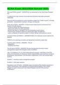
A histogram provides information about the distribution of the values:
1. Location (Central tendency, Median, Mode, Mean) 2 distributions with
different locations.
2. Spread (Variability) 2 distributions with different spreads.
3. Skewness (lack of symmetry)
4. Kurtosis (thick and long tails)
5. Outliers (remote (afgezonderde) values)
, 6. Special features (e.g. gaps in the data)
Percentiles
80th percentile = score with 80% cumulative percentage (80% below and 20%
of the scores above it).
Quartiles:
The 1st and 3rd quartile are called Turkey’s Hinges. The 2nd quartile is called the
Median.
Q1: first quartile: 25th percentile if n is odd use the lower half including the median.
Q2: second quartile: 50th percentile if n is even the Median is the midway between the 2 values.
Q3: third quartile: 75th percentile if n is odd use the upper half including the median.
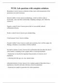
Reading a Box plot:
1 - Location (central tendency) - median, Q2
2 - Spread (variability) - length of box (IQR)= Q3 –
Q1
3 - Skewness (no symmetry) - compare
whiskers & outliers
4 - Length of tails - difficult to judge
5 - Outliers - indicated individually
Measure of central tendency, or sample mean (or
average) – similar to population mean:
Range = Maximum score – Minimum score
Measure the spread of observations around the
central tendency.
Variance average of the squared differences between each
observation and the mean:
Standard Deviation: Square root of the variance:
The useful distance of the observation to the sample mean. So it
measures the spread of the observations.
A larger variances makes it harder to predict an individual
value of the variable
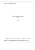
Skewness: the measure of asymmetry of a distribution (is one tail longer than the other?):
Values outside -1, 1 indicate serious skew
Positive skewness: Sample Mean > Median
Negative skewness: Sample Mean < Median
Efficient statistics (actually use all statistics): Mean, Standard
Deviation, Skewness
Inefficient statistics: Median, mode, IQR, Range
(Sensitive to
outliers)
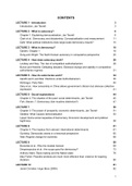
Z-score: The amount of standard deviations a score is above/below the sample
mean:
Z-score ouside (-2,5; 2,5) indicates an outlier.
, If the lowest score lies less than 1 SD from the mean it indicates positive skewness and vice
versa.
If the distribution is bell-shaped, then approximately:
5% of the observations has zi < -1.645 and 5% has zi > 1.645
2.5% of the observations has zi< -1.96 and 2.5% has zi > 1.96
0.5% of the observations has zi< -2.576 and 0.5% has zi > 2.576
The sample statistics provide information about the distribution of the values:
1 Location (central tendency) → mean, median, mode
2 Spread (variability) → standard deviation, IQR, range
3 Skewness (lack of symmetry) → skewness
4 Kurtosis (thick and long tails) → not covered in this course
5 Outliers → see z-scores
Requirements for the variables:
Bell-shaped (strong requirement)
Symmetrical distribution (weak requirement)
Lessons learned
Homework exercises:
If there is asked to give Q2 of a variable and the n= even (e.g. 68). Q2 = (x34+
x35)/2.
o For Q1 and Q3 if n = even (68) take the middle of the first/last half including
Q2. So in this case35/2 is (x17 + x18)/2 = Q1.
After calculating the variance DON’T FORGET to Root the variance to calculate SD!
If the Mean > Median positive skew and vice versa.
Skewness is not a valid statistic for Ordinal data.
Mode and median are valid statistics for Ordinal data.
o Mode IS and Median IS NOT a valid statistic for nominal data.
In case one is asking to interpret the spread it is calculated with the IQR.
High/positive kurtosis is presence if both whiskers are relatively long (longer than
the box).
The distribution is positively skewed if the upper whisker is longer than the other
(Boxplot).
The distribution is positively skewed if the bars left in the histogram are higher than
right.
Additional exercises:
2b. If they ask relative frequency number/total don’t give percentages just
give e.g. 0.16.
2b. You would use a histogram instead of a bar chart because the spaces between
the bars (with a bar chart) would suggest the value between the bars are not
possible.
The type of statistical analysis depends on the type of variable
QUALITATIVE variable: outcomes are categories
4. Nominal: unordered categories (Male/Female)
3. Categorical: ordered categories (Likert scale, Job skill)
QUANTITATIVE variables: outcomes are numbers
2. Discrete: series of isolated numbers (numbers of cars sold, change in
employees)
1. Continuous: interval of possible values (BNP, temperature)
A variable can always be treated as a lower type.
For QUALITATIVE data we use:
Pie chart (suited for ordinal data)
Bar chart (suited for ordinal data)
Frequency table Note: cumulative 50% is the Median.
Median (the middle outcome only for ordinal data)
Mode (the most frequent number)
For QUANTITATIVE data we use:
Histogram (the highest bar in the graph is the Mode)
Mode, Range
Percentiles, including Median and Quartiles
Boxplot
Mean, Standard deviation, Kurtosis, Skewness
Z-scores
Likert variable cannot be treated as quantitative (then one would
assume that the differences between the scales are similar,
which is not).
Binary variable is a categorical variable consisting of 2 categories (k=2) can always be
treated as nominal, categorical and discrete (Male / Female)
A histogram provides information about the distribution of the values:
1. Location (Central tendency, Median, Mode, Mean) 2 distributions with
different locations.
2. Spread (Variability) 2 distributions with different spreads.
3. Skewness (lack of symmetry)
4. Kurtosis (thick and long tails)
5. Outliers (remote (afgezonderde) values)
, 6. Special features (e.g. gaps in the data)
Percentiles
80th percentile = score with 80% cumulative percentage (80% below and 20%
of the scores above it).
Quartiles:
The 1st and 3rd quartile are called Turkey’s Hinges. The 2nd quartile is called the
Median.
Q1: first quartile: 25th percentile if n is odd use the lower half including the median.
Q2: second quartile: 50th percentile if n is even the Median is the midway between the 2 values.
Q3: third quartile: 75th percentile if n is odd use the upper half including the median.
Reading a Box plot:
1 - Location (central tendency) - median, Q2
2 - Spread (variability) - length of box (IQR)= Q3 –
Q1
3 - Skewness (no symmetry) - compare
whiskers & outliers
4 - Length of tails - difficult to judge
5 - Outliers - indicated individually
Measure of central tendency, or sample mean (or
average) – similar to population mean:
Range = Maximum score – Minimum score
Measure the spread of observations around the
central tendency.
Variance average of the squared differences between each
observation and the mean:
Standard Deviation: Square root of the variance:
The useful distance of the observation to the sample mean. So it
measures the spread of the observations.
A larger variances makes it harder to predict an individual
value of the variable
Skewness: the measure of asymmetry of a distribution (is one tail longer than the other?):
Values outside -1, 1 indicate serious skew
Positive skewness: Sample Mean > Median
Negative skewness: Sample Mean < Median
Efficient statistics (actually use all statistics): Mean, Standard
Deviation, Skewness
Inefficient statistics: Median, mode, IQR, Range
(Sensitive to
outliers)
Z-score: The amount of standard deviations a score is above/below the sample
mean:
Z-score ouside (-2,5; 2,5) indicates an outlier.
, If the lowest score lies less than 1 SD from the mean it indicates positive skewness and vice
versa.
If the distribution is bell-shaped, then approximately:
5% of the observations has zi < -1.645 and 5% has zi > 1.645
2.5% of the observations has zi< -1.96 and 2.5% has zi > 1.96
0.5% of the observations has zi< -2.576 and 0.5% has zi > 2.576
The sample statistics provide information about the distribution of the values:
1 Location (central tendency) → mean, median, mode
2 Spread (variability) → standard deviation, IQR, range
3 Skewness (lack of symmetry) → skewness
4 Kurtosis (thick and long tails) → not covered in this course
5 Outliers → see z-scores
Requirements for the variables:
Bell-shaped (strong requirement)
Symmetrical distribution (weak requirement)
Lessons learned
Homework exercises:
If there is asked to give Q2 of a variable and the n= even (e.g. 68). Q2 = (x34+
x35)/2.
o For Q1 and Q3 if n = even (68) take the middle of the first/last half including
Q2. So in this case35/2 is (x17 + x18)/2 = Q1.
After calculating the variance DON’T FORGET to Root the variance to calculate SD!
If the Mean > Median positive skew and vice versa.
Skewness is not a valid statistic for Ordinal data.
Mode and median are valid statistics for Ordinal data.
o Mode IS and Median IS NOT a valid statistic for nominal data.
In case one is asking to interpret the spread it is calculated with the IQR.
High/positive kurtosis is presence if both whiskers are relatively long (longer than
the box).
The distribution is positively skewed if the upper whisker is longer than the other
(Boxplot).
The distribution is positively skewed if the bars left in the histogram are higher than
right.
Additional exercises:
2b. If they ask relative frequency number/total don’t give percentages just
give e.g. 0.16.
2b. You would use a histogram instead of a bar chart because the spaces between
the bars (with a bar chart) would suggest the value between the bars are not
possible.