May 21, 2020 APM346 – Week 3 Justin Ko
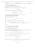
1 The Wave Equation on R
The one dimensional wave equation models a vibrating string.
Definition 1. For parameters c ∈ R+ , the homogeneous wave equation on R × R+ is
utt − c2 uxx = 0. (1)
The corresponding IVP for the inhomogeneous wave equation is
2
utt − c uxx = f (x, t)
x ∈ R, t > 0,
u|t=0 = g(x) x ∈ R, (2)
ut |t=0 = h(x) x ∈ R.
The solution to this equation is derived using the method of characteristics.
Theorem 1 (Solution to the Wave Equation)
(a) The general solution to (1) is
u(x, t) = φ(x − ct) + ψ(x + ct), (3)
where φ, ψ are arbitrary functions.
(b) The particular solution to (2) is given by d’Alembert’s Formula,
x+ct Z tZ x+c(t−s)
g(x + ct) + g(x − ct)
Z
1 1
u(x, t) = + h(s) ds + f (y, s) dyds. (4)
2 2c x−ct 2c 0 x−c(t−s)
1.1 Derivation of the General Solution
We give two derivations of the general solution (3).
1.1.1 Method 1: Factoring the Operator
We reduce the second order PDE to iterated first order PDEs and apply the methods from Week 2.
We begin by factoring the linear operator L[u] = (∂t2 − c2 ∂x2 )u,
L[u] = (∂t2 − c2 ∂x2 )u = (∂t + c∂x )(∂t − c∂x )u.
Notice that if u is a solution to (1), then L[u] = 0. If we define v = (∂t − c∂x )u = ut − cux , then
L[u] = 0 ⇐⇒ (∂t + c∂x )(∂t − c∂x )u = (∂t + c∂x )v = vt + cvx = 0.
This gives us the following system of first order equations
(
ut − cux = v
. (5)
vt + cvx = 0
Solving the Second Equation: Using the general solution of the transport equation (see Week 2),
vt + cvx = 0 =⇒ v(x, t) = ϕ0 (x − ct)
Page 1 of 12
, May 21, 2020 APM346 – Week 3 Justin Ko
for some differentiable function ϕ0 (this form was chosen to simplify notation).
Solving the First Equation: Since v = ut − cux to recover u, we need to solve
ut − cux = ϕ0 (x − ct).
This is a first order linear equation, so it suffices to solve the system
dt dx du
= = 0 .
1 −c ϕ (x − ct)
The equation involving the first and second terms gives us the characteristics
dt dx
= =⇒ x = −ct + C =⇒ C = x + ct.
1 −c
Solving the equation involving the first third term implies
dt du du 1 1
= 0 = 0 =⇒ u(x, t) = − ϕ(C − 2ct) + ψ(C) = − ϕ(x − ct) + ψ(x + ct).
1 ϕ (x − ct) ϕ (C − 2ct) 2c 2c
1
If we define φ = − 2c ϕ, then we get the general solution
u(x, t) = φ(x − ct) + ψ(x + ct).
1.1.2 Method 2: Change of Variables
We do a change of variables to simplify the form of the PDE. We begin by factoring the linear operator
L[u] = (∂t2 − c2 ∂x2 )u,
L[u] = (∂t2 − c2 ∂x2 )u = (∂t + c∂x )(∂t − c∂x )u.
This factorization seems to suggest two characteristic curves
dt dx dt dx
= =⇒ C = x − ct and = =⇒ D = x + ct.
1 c 1 −c
We will use these characteristics curves to define a change of variables that will greatly simplify the
PDE. Consider the change of variables
ξ(x, t) = x − ct and η(x, t) = x + ct. (6)
By the multivariable chain rule,
∂u ∂ξ ∂u ∂η
∂t u(ξ, η) = · + · = −cuξ + cuη = (−c∂ξ + c∂η )u(ξ, η) =⇒ ∂t = (−c∂ξ + c∂η )
∂ξ ∂t ∂η ∂t
and
∂u ∂ξ ∂u ∂η
∂x u(ξ, η) = · + · = uξ + uη = (∂ξ + ∂η )u(ξ, η) =⇒ ∂x = (∂ξ + ∂η ).
∂ξ ∂x ∂η ∂x
In particular, these computations imply that the original operators are equal to
(∂t + c∂x ) = ((−c∂ξ + c∂η ) + c(∂ξ + ∂η )) = 2c∂η
and
(∂t − c∂x ) = ((−c∂ξ + c∂η ) − c(∂ξ + ∂η )) = −2c∂ξ .
Therefore, under the change of variables (6),
L[u] = (∂t2 − c2 ∂x2 )u = (∂t + c∂x )(∂t − c∂x )u = (2c∂η )(−2c∂ξ )u = −4c2 uξη .
If u satisfies (1), then L[u] = 0. Since c 6= 0, directly integrating this PDE (see Week 1) implies
0 = L[u] = −4c2 uξη =⇒ u(ξ, η) = φ(ξ) + ψ(η) =⇒ u(x, t) = φ(x − ct) + ψ(x + ct),
after writing it back in the original variables using (6).
Remark 1. From the proofs, we see that the general solution (3) holds for t < 0 as well.
Page 2 of 12
1 The Wave Equation on R
The one dimensional wave equation models a vibrating string.
Definition 1. For parameters c ∈ R+ , the homogeneous wave equation on R × R+ is
utt − c2 uxx = 0. (1)
The corresponding IVP for the inhomogeneous wave equation is
2
utt − c uxx = f (x, t)
x ∈ R, t > 0,
u|t=0 = g(x) x ∈ R, (2)
ut |t=0 = h(x) x ∈ R.
The solution to this equation is derived using the method of characteristics.
Theorem 1 (Solution to the Wave Equation)
(a) The general solution to (1) is
u(x, t) = φ(x − ct) + ψ(x + ct), (3)
where φ, ψ are arbitrary functions.
(b) The particular solution to (2) is given by d’Alembert’s Formula,
x+ct Z tZ x+c(t−s)
g(x + ct) + g(x − ct)
Z
1 1
u(x, t) = + h(s) ds + f (y, s) dyds. (4)
2 2c x−ct 2c 0 x−c(t−s)
1.1 Derivation of the General Solution
We give two derivations of the general solution (3).
1.1.1 Method 1: Factoring the Operator
We reduce the second order PDE to iterated first order PDEs and apply the methods from Week 2.
We begin by factoring the linear operator L[u] = (∂t2 − c2 ∂x2 )u,
L[u] = (∂t2 − c2 ∂x2 )u = (∂t + c∂x )(∂t − c∂x )u.
Notice that if u is a solution to (1), then L[u] = 0. If we define v = (∂t − c∂x )u = ut − cux , then
L[u] = 0 ⇐⇒ (∂t + c∂x )(∂t − c∂x )u = (∂t + c∂x )v = vt + cvx = 0.
This gives us the following system of first order equations
(
ut − cux = v
. (5)
vt + cvx = 0
Solving the Second Equation: Using the general solution of the transport equation (see Week 2),
vt + cvx = 0 =⇒ v(x, t) = ϕ0 (x − ct)
Page 1 of 12
, May 21, 2020 APM346 – Week 3 Justin Ko
for some differentiable function ϕ0 (this form was chosen to simplify notation).
Solving the First Equation: Since v = ut − cux to recover u, we need to solve
ut − cux = ϕ0 (x − ct).
This is a first order linear equation, so it suffices to solve the system
dt dx du
= = 0 .
1 −c ϕ (x − ct)
The equation involving the first and second terms gives us the characteristics
dt dx
= =⇒ x = −ct + C =⇒ C = x + ct.
1 −c
Solving the equation involving the first third term implies
dt du du 1 1
= 0 = 0 =⇒ u(x, t) = − ϕ(C − 2ct) + ψ(C) = − ϕ(x − ct) + ψ(x + ct).
1 ϕ (x − ct) ϕ (C − 2ct) 2c 2c
1
If we define φ = − 2c ϕ, then we get the general solution
u(x, t) = φ(x − ct) + ψ(x + ct).
1.1.2 Method 2: Change of Variables
We do a change of variables to simplify the form of the PDE. We begin by factoring the linear operator
L[u] = (∂t2 − c2 ∂x2 )u,
L[u] = (∂t2 − c2 ∂x2 )u = (∂t + c∂x )(∂t − c∂x )u.
This factorization seems to suggest two characteristic curves
dt dx dt dx
= =⇒ C = x − ct and = =⇒ D = x + ct.
1 c 1 −c
We will use these characteristics curves to define a change of variables that will greatly simplify the
PDE. Consider the change of variables
ξ(x, t) = x − ct and η(x, t) = x + ct. (6)
By the multivariable chain rule,
∂u ∂ξ ∂u ∂η
∂t u(ξ, η) = · + · = −cuξ + cuη = (−c∂ξ + c∂η )u(ξ, η) =⇒ ∂t = (−c∂ξ + c∂η )
∂ξ ∂t ∂η ∂t
and
∂u ∂ξ ∂u ∂η
∂x u(ξ, η) = · + · = uξ + uη = (∂ξ + ∂η )u(ξ, η) =⇒ ∂x = (∂ξ + ∂η ).
∂ξ ∂x ∂η ∂x
In particular, these computations imply that the original operators are equal to
(∂t + c∂x ) = ((−c∂ξ + c∂η ) + c(∂ξ + ∂η )) = 2c∂η
and
(∂t − c∂x ) = ((−c∂ξ + c∂η ) − c(∂ξ + ∂η )) = −2c∂ξ .
Therefore, under the change of variables (6),
L[u] = (∂t2 − c2 ∂x2 )u = (∂t + c∂x )(∂t − c∂x )u = (2c∂η )(−2c∂ξ )u = −4c2 uξη .
If u satisfies (1), then L[u] = 0. Since c 6= 0, directly integrating this PDE (see Week 1) implies
0 = L[u] = −4c2 uξη =⇒ u(ξ, η) = φ(ξ) + ψ(η) =⇒ u(x, t) = φ(x − ct) + ψ(x + ct),
after writing it back in the original variables using (6).
Remark 1. From the proofs, we see that the general solution (3) holds for t < 0 as well.
Page 2 of 12