Onderzoeksvaardigheden II – Tutorials
Module 1
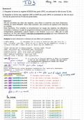
#Package “gmodels” for tables
Library(gmodels)
Library(ggplot2)
Library(stargazer)
Library(psych)
dir <- "~/Documents/ERASMUS
RSM/Onderzoeksvaardigheden/Tutorials/Data" /"
dirData <- paste0(dir, "Data/")
dirProg <- paste0(dir, "Programs/")
dirRslt <- paste0(dir, "Results/")
Ontbrekende waarden / missing values:
colSums(is.na(dsTitanic))
DATA FACTORS
dsLiving$fLiving <- factor(dsLiving$cLiving, levels=c(1:5), labels=c(“Student housing”,
“Private rent”, “Parents”, “Own house”, “Other”))
levels(dsLiving$fLiving)
when you turn it into a factor then you have to specify the number of outcomes that’s where
the “levels” is for. R understands that this is categorical data, which is necessary when later
on making use of graphics or other analyses.
FREQUENCY TABLES AND VISUALISATION
Visualization of the information between two qualitative variables
#Frequency table
Use of function tables
Table(dsLiving$cLiving)
Table(dsLiving$fFraternity)
Table(‘living situation’ = dsLiving$fLiving, Membership = dsLiving$dFraternity)
#Use of function xtabs
It generates the same table, but operates different. Structured and layout.
Tbl <- xtabs( ~ cLiving + dFraternity, data = dsLiving)
#make a table with margins totals (as in the slides of Module 1, totals of rows and columns)
Addmargins(tbl)
,#GGplot for these tables bij sommige data neemt de x-as niet optie 1 of 2 maar een
numerieke maat, dit is fout.
Ggplot(dsLiving, aes(x = fliving)) + geom_bar(fill = “orange”, col= “black”) + xlab(“Living
conditions (cliving)”)
Ggsave(paste0(dirRslt, “Tutorial01.pdf”), width = 8, height = 6)
#make grouped tables/bar charts with GGplot
Ggplot(dsLiving, aes(x=fFraternity, fill=fliving)) + geombar(position= “dodge”) +
ylab(“Frequentie”) + xlab(“Lidmaatschap”) + scale_fill_brewer(“Woonsituatie”, palette=
“Set1”)
Ggsave function
The dodge function makes the table put the data next to each other instead of stacked on
top of each other, which makes it easier to interpret data. Woonsituatie is stating the legend
and the colours the bars will have.
ANALYSIS OF STATISTICAL INDEPENDENCE between 2 qualitative variables (categorical data)
#Chi square test
Step 1 make a frequency table
Tbl <- table(dsLiving$cliving, dsLiving$dFraternity)
Step 2 the chi square test
Chisq.test(tbl) 1st value is observed value, degrees of freedom & p-value. The approximation
of the Chisquare test is better the larger the sample size (observed values). (rule of 5!)
However, this cannot be checked by the frequency tables because these are observed and
not the expected frequencies.
Step 3 extract information from object. To check the expected frequencies
RsltChisq <- chisq.test(tbl)
Str(rsltChisq)
With this you can already see the observed and expected values
rsltChisq$statistic observed value of the statistic
rsltChisq$parameter degrees of freedom
rsltChisq$p.value p-value
round(cbind(rsltChisq$observed, rsltChisq$expected, 3)
Step 4 find cells with expected frequencies below 5 OPTION 1
Which(rsltChisq$expected < 5)
Which(rsltChisq$expected < 5, arr.ind = TRUE) arr.ind makes it more clear which row and
column the value below 5 is in
, Step 5 remove rows with sparse outcomes reanalyse the relationship between the variables.
dsLiving.tmp <- dsLiving[!(dsLiving$cLiving ==5), c(“cLiving”, “dFraternity”)]
Step 6 re-make the frequency table
Tbl <- table(dsLiving.tmp$cLiving, dsLiving$dFraternity)
Step 7 Find the chi-square test results
Chisq.test(tbl)
The warning message will not show anymore.
OPTION 2 – combining rows with sparse outcomes (to leave out <5)
Step 1 – copy data to temporary data frame
DsLiving.tmp <- dsLiving[c(“cLiving”, “dFraternity”)]
Step 2- adjust the value
dsLiving.tmp$cLiving[dsLiving.tmp$cLiving==5] <-4 combining outcome 5 with outcome 4
Step 3 – remake the frequency table
Tbl <- table(dsLiving.tmp$cLiving, dsLiving.tmp$dFraternity)
Step 4 – Find the chisquare test results
Chisq.test(tbl)
Also no warning message.
#if the expected frequencies are falling short of the rule of 5 then we cannot use chisq and
you cannot combine rows/columns with a 2x2 table and all expected values are above 5
Yates continuity correction - contingency analysis
Step 1 make a frequency table
Tbl <- table(dsLiving$dSports, dsLiving$dFraternity)
Step 2 Find the chisq test results
Chisq.test(tbl)
Tmp <- chisq.test(tbl)
Step 3 use phi see slides for uitleg
Phi <- sqrt(tmp$statistic/sum(tbl))
R automatically applies this correction of ½ in the formula.
# 2x2 table but the expected values are still below 5
Fisher’s exact test
Step 1 make a frequency table
Tbl <- table(dsLiving$dSports, dsLiving$dFraternity)
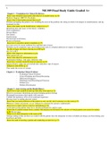
Module 1
#Package “gmodels” for tables
Library(gmodels)
Library(ggplot2)
Library(stargazer)
Library(psych)
dir <- "~/Documents/ERASMUS
RSM/Onderzoeksvaardigheden/Tutorials/Data" /"
dirData <- paste0(dir, "Data/")
dirProg <- paste0(dir, "Programs/")
dirRslt <- paste0(dir, "Results/")
Ontbrekende waarden / missing values:
colSums(is.na(dsTitanic))
DATA FACTORS
dsLiving$fLiving <- factor(dsLiving$cLiving, levels=c(1:5), labels=c(“Student housing”,
“Private rent”, “Parents”, “Own house”, “Other”))
levels(dsLiving$fLiving)
when you turn it into a factor then you have to specify the number of outcomes that’s where
the “levels” is for. R understands that this is categorical data, which is necessary when later
on making use of graphics or other analyses.
FREQUENCY TABLES AND VISUALISATION
Visualization of the information between two qualitative variables
#Frequency table
Use of function tables
Table(dsLiving$cLiving)
Table(dsLiving$fFraternity)
Table(‘living situation’ = dsLiving$fLiving, Membership = dsLiving$dFraternity)
#Use of function xtabs
It generates the same table, but operates different. Structured and layout.
Tbl <- xtabs( ~ cLiving + dFraternity, data = dsLiving)
#make a table with margins totals (as in the slides of Module 1, totals of rows and columns)
Addmargins(tbl)
,#GGplot for these tables bij sommige data neemt de x-as niet optie 1 of 2 maar een
numerieke maat, dit is fout.
Ggplot(dsLiving, aes(x = fliving)) + geom_bar(fill = “orange”, col= “black”) + xlab(“Living
conditions (cliving)”)
Ggsave(paste0(dirRslt, “Tutorial01.pdf”), width = 8, height = 6)
#make grouped tables/bar charts with GGplot
Ggplot(dsLiving, aes(x=fFraternity, fill=fliving)) + geombar(position= “dodge”) +
ylab(“Frequentie”) + xlab(“Lidmaatschap”) + scale_fill_brewer(“Woonsituatie”, palette=
“Set1”)
Ggsave function
The dodge function makes the table put the data next to each other instead of stacked on
top of each other, which makes it easier to interpret data. Woonsituatie is stating the legend
and the colours the bars will have.
ANALYSIS OF STATISTICAL INDEPENDENCE between 2 qualitative variables (categorical data)
#Chi square test
Step 1 make a frequency table
Tbl <- table(dsLiving$cliving, dsLiving$dFraternity)
Step 2 the chi square test
Chisq.test(tbl) 1st value is observed value, degrees of freedom & p-value. The approximation
of the Chisquare test is better the larger the sample size (observed values). (rule of 5!)
However, this cannot be checked by the frequency tables because these are observed and
not the expected frequencies.
Step 3 extract information from object. To check the expected frequencies
RsltChisq <- chisq.test(tbl)
Str(rsltChisq)
With this you can already see the observed and expected values
rsltChisq$statistic observed value of the statistic
rsltChisq$parameter degrees of freedom
rsltChisq$p.value p-value
round(cbind(rsltChisq$observed, rsltChisq$expected, 3)
Step 4 find cells with expected frequencies below 5 OPTION 1
Which(rsltChisq$expected < 5)
Which(rsltChisq$expected < 5, arr.ind = TRUE) arr.ind makes it more clear which row and
column the value below 5 is in
, Step 5 remove rows with sparse outcomes reanalyse the relationship between the variables.
dsLiving.tmp <- dsLiving[!(dsLiving$cLiving ==5), c(“cLiving”, “dFraternity”)]
Step 6 re-make the frequency table
Tbl <- table(dsLiving.tmp$cLiving, dsLiving$dFraternity)
Step 7 Find the chi-square test results
Chisq.test(tbl)
The warning message will not show anymore.
OPTION 2 – combining rows with sparse outcomes (to leave out <5)
Step 1 – copy data to temporary data frame
DsLiving.tmp <- dsLiving[c(“cLiving”, “dFraternity”)]
Step 2- adjust the value
dsLiving.tmp$cLiving[dsLiving.tmp$cLiving==5] <-4 combining outcome 5 with outcome 4
Step 3 – remake the frequency table
Tbl <- table(dsLiving.tmp$cLiving, dsLiving.tmp$dFraternity)
Step 4 – Find the chisquare test results
Chisq.test(tbl)
Also no warning message.
#if the expected frequencies are falling short of the rule of 5 then we cannot use chisq and
you cannot combine rows/columns with a 2x2 table and all expected values are above 5
Yates continuity correction - contingency analysis
Step 1 make a frequency table
Tbl <- table(dsLiving$dSports, dsLiving$dFraternity)
Step 2 Find the chisq test results
Chisq.test(tbl)
Tmp <- chisq.test(tbl)
Step 3 use phi see slides for uitleg
Phi <- sqrt(tmp$statistic/sum(tbl))
R automatically applies this correction of ½ in the formula.
# 2x2 table but the expected values are still below 5
Fisher’s exact test
Step 1 make a frequency table
Tbl <- table(dsLiving$dSports, dsLiving$dFraternity)