Solutions 37
Chapter 1 Solutions
1.1. (a) Gender is categorical. (b) Age is quantitative. (c) Race is categorical.
(d) Smoker is categorical. (e) Blood pressure is quantitative. (f ) Calcium level is
quantitative.
1.2. (a) The individuals in this exercise are the different brands of breakfast cereals.
(b) The variables are manufacturer (categorical), preparation method (categorical),
calories (quantitative), sugar content (quantitative), and fiber content (quantitative).
30
1.3. (a) Shown on the right. (b) A
pie chart would not be appro- 25
priate because the data for the 20
Percent smoking
four groups do not make up one
15
whole. Making two pie charts
would not work either, for the 10
same reason. Instead, the percent 5
who smoke in any given group
is complementary to the percent 0
Men 18-24 years Women 18-24 years Men 25-29 years Women 25-29 years
who do not smoke in that given
group.
1.4. A pie chart could also be made, 16,000
but the relative heights of the bars 14,000
are easier to compare than the 12,000
Number of births
relative sizes of the “slices” of the 10,000
pie. 8,000
The most likely explanation 6,000
for the lower weekend numbers is 4,000
2,000
that, when a birth is “planned”
0
(either by inducement or cesarean Sun Mon Tue Wed Thu Fri Sat
section), it is usually scheduled for
a weekday—perhaps more due to the preferences of the physician or midwife.
1.5. Some statistical programs automatically include the lower end of each class while
excluding the upper end, and other programs automatically include the upper end of
each class while excluding the lower end. The histogram below on the left includes the
upper boundary of each class, whereas the histogram below on the right includes the
lower boundary. Either way is fine, but you should always be sure to understand how
your software package defines the classes in your histogram.
,38 Chapter 1 Picturing Distributions with Graphs
5 4
4
3
Frequency
Frequency
3
2
2
1
1
0 0
10 15 20 25 30 35 40 45 10 15 20 25 30 35 40 45
Healing rate (micrometers per hour) Healing rate (micrometers per hour)
1.6. (a) The applet creates a histogram with 7 classes. (b) It is possible to get to one
class ranging from 11 to 41 (not a very useful histogram). (c) The most classes the
applet will allow is 15; the classes with the highest count have only 2 observations.
(d) Choices will vary; anything from about 6 to 10 classes is reasonable. A sample size
of only 18 can be a little awkward to fit in a histogram, because even small changes in
class choice can have a substantial impact on the overall look of the histogram.
1.7. Overall, the histogram is somewhat symmetric and unimodal. However, the dataset
is not very large and it makes it harder to conclude. For example, the large first class
of the histogram could reflect either some minor fluctuation or an underlying bimodal
trend.
1.8. The histogram is clearly unimodal and symmetric, without outliers. The midpoint
lies in the 14-to-15-years class, which represents 14-year-old girls.
1.9. (a) Shown are two versions of this stemplot. For 0 8 0 799
the first, we have (as the text suggests) rounded 1 000134 1 0134444
1 5555677 1 5577
to the nearest 10; for the second, we have trimmed 2 0 2 0
numbers (dropped the last digit). 359 mg/dl appears 2 67 2 57
to be an outlier. The stemplot is unimodal and 3 3
slightly right-skewed (even if we ignore the outlier). 3 6 3 5
Overall, glucose levels are not under control: Only 4 of the 18 had levels in the desired
range. (b) The midpoint is between 147 and 148 and the spread is from 78 to 359.
(c) The dotplot (shown below) and the stemplot are very similar, but the dotplot
shows the exact location of each data point and is therefore a little bit more detailed.
,Solutions 39
1.10. The back-to-back stemplot displays the glucose levels Individual Group
for the individual instruction group on the left and for the 0 799
class instruction group on the right. As with Exercise 1.9, 22 1 0134444
two versions of the stemplots are shown. For the first, we 99866655 2 5577
have (as the text suggests) rounded to the nearest 10; for 22222 2 0
the second, we have trimmed numbers (dropped the last 8 3 57
digit). Both distributions are unimodal. Glucose levels in 3
3 5
the individual instruction group are less variable and appear
symmetric without outliers. Overall, most individuals in 0 8
both groups have glucose levels that are not adequately 33 1 000134
controlled. 966666 2 5555677
3322200 2 0
8 3 67
3
3 6
40
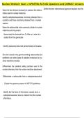
1.11. The timeplot shows a clear decrease
35
in the percent of childbirths using routine
episiotomy—suggesting a slow but steady 30
change in hospital birthing practices.
Percent of childbirths
25
20
15
10
5
0
1998 2000 2002 2004 2006 2008 2010
1.12. The data have both an obvious overall trend and clear cyclical variations. Monthly
CO2 levels vary seasonally, peaking in the spring and bottoming in the fall, creating
annual cycles. But the big picture shows a clear upward trend reflecting increasing
monthly CO2 levels over the full forty-year period for which data exist. This suggests
that we should think carefully about our global carbon emission and possible action
courses.
1.13. (c) Sex is categorical (can only be male or female) and weight is quantitative (a
numerical value that can be averaged for multiple bear cubs).
1.14. (c) The data can be displayed either on a pie chart or a bar graph because the
categories represent the pieces of a whole.
1.15. (a) Kidney transplants represented nearly 61% (16,624/27,463) of all single-organ
transplants in 2007.
1.16. (a) The right-most bar represents 4 perch.
1.17. (b) The right-most bar represents perch with lengths ranging from about 45.1 to
50 cm.
, 40 Chapter 1 Picturing Distributions with Graphs
1.18. (b) The stems should be the first two digits.
1.19. (b) The highest percent is 17.6% (a stem of 17, with leaf 0.6).
1.20. (b) The distribution is somewhat symmetric to slightly left-skewed.
1.21. (a) The 25th and 26th percents are 12.7% and 12.8%.
1.22. (a) The distribution is skewed to the left because most individuals diagnosed with
multiple myeloma are old and few are young.
1.23. (a) Number of eggs is quantitative, a count. (b) Incubation period is quantitative,
a length of time. (c) Parental care is categorical, 1 of only 3 possible choices. (d) Nest
size is quantitative, a measure of size. (e) Presence of pesticides is categorical, 1 of
only 2 possible choices.
1.24. Answers will vary. Examples of categorical variables are gender (boy/girl), lunch
type (school provided/ home prepared), and milk consumption (yes/no). Examples of
quantitative variables are age (in years), approximate number of calories consumed on
the day before the interview (in Calories), and typical number of fruit and vegetable
servings per day (a unitless count).
1.25. (a) The 53 lakes are the individuals. (b) There are 5 variables recorded, 4
quantitative and 1 categorical (age of data). Age of data is categorical because the
only possible entries are recent data and year-old data (non-numerical).
1.26. (a) Shown below. (b) In order to make a pie chart, we would need to know the
total number of deaths in this age group (so that we could compute the number of
deaths due to other causes).
16 16
14 14
Thousands of deaths
Thousands of deaths
12 12
10 10
8 8
6 6
4 4
2 2
0 0
Accidents
Congenital
Homicide
Cancer
disease
Suicide
Accidents
Congenital
Cancer
disease
Homicide
Suicide
Heart
Heart
defects
defects
Chapter 1 Solutions
1.1. (a) Gender is categorical. (b) Age is quantitative. (c) Race is categorical.
(d) Smoker is categorical. (e) Blood pressure is quantitative. (f ) Calcium level is
quantitative.
1.2. (a) The individuals in this exercise are the different brands of breakfast cereals.
(b) The variables are manufacturer (categorical), preparation method (categorical),
calories (quantitative), sugar content (quantitative), and fiber content (quantitative).
30
1.3. (a) Shown on the right. (b) A
pie chart would not be appro- 25
priate because the data for the 20
Percent smoking
four groups do not make up one
15
whole. Making two pie charts
would not work either, for the 10
same reason. Instead, the percent 5
who smoke in any given group
is complementary to the percent 0
Men 18-24 years Women 18-24 years Men 25-29 years Women 25-29 years
who do not smoke in that given
group.
1.4. A pie chart could also be made, 16,000
but the relative heights of the bars 14,000
are easier to compare than the 12,000
Number of births
relative sizes of the “slices” of the 10,000
pie. 8,000
The most likely explanation 6,000
for the lower weekend numbers is 4,000
2,000
that, when a birth is “planned”
0
(either by inducement or cesarean Sun Mon Tue Wed Thu Fri Sat
section), it is usually scheduled for
a weekday—perhaps more due to the preferences of the physician or midwife.
1.5. Some statistical programs automatically include the lower end of each class while
excluding the upper end, and other programs automatically include the upper end of
each class while excluding the lower end. The histogram below on the left includes the
upper boundary of each class, whereas the histogram below on the right includes the
lower boundary. Either way is fine, but you should always be sure to understand how
your software package defines the classes in your histogram.
,38 Chapter 1 Picturing Distributions with Graphs
5 4
4
3
Frequency
Frequency
3
2
2
1
1
0 0
10 15 20 25 30 35 40 45 10 15 20 25 30 35 40 45
Healing rate (micrometers per hour) Healing rate (micrometers per hour)
1.6. (a) The applet creates a histogram with 7 classes. (b) It is possible to get to one
class ranging from 11 to 41 (not a very useful histogram). (c) The most classes the
applet will allow is 15; the classes with the highest count have only 2 observations.
(d) Choices will vary; anything from about 6 to 10 classes is reasonable. A sample size
of only 18 can be a little awkward to fit in a histogram, because even small changes in
class choice can have a substantial impact on the overall look of the histogram.
1.7. Overall, the histogram is somewhat symmetric and unimodal. However, the dataset
is not very large and it makes it harder to conclude. For example, the large first class
of the histogram could reflect either some minor fluctuation or an underlying bimodal
trend.
1.8. The histogram is clearly unimodal and symmetric, without outliers. The midpoint
lies in the 14-to-15-years class, which represents 14-year-old girls.
1.9. (a) Shown are two versions of this stemplot. For 0 8 0 799
the first, we have (as the text suggests) rounded 1 000134 1 0134444
1 5555677 1 5577
to the nearest 10; for the second, we have trimmed 2 0 2 0
numbers (dropped the last digit). 359 mg/dl appears 2 67 2 57
to be an outlier. The stemplot is unimodal and 3 3
slightly right-skewed (even if we ignore the outlier). 3 6 3 5
Overall, glucose levels are not under control: Only 4 of the 18 had levels in the desired
range. (b) The midpoint is between 147 and 148 and the spread is from 78 to 359.
(c) The dotplot (shown below) and the stemplot are very similar, but the dotplot
shows the exact location of each data point and is therefore a little bit more detailed.
,Solutions 39
1.10. The back-to-back stemplot displays the glucose levels Individual Group
for the individual instruction group on the left and for the 0 799
class instruction group on the right. As with Exercise 1.9, 22 1 0134444
two versions of the stemplots are shown. For the first, we 99866655 2 5577
have (as the text suggests) rounded to the nearest 10; for 22222 2 0
the second, we have trimmed numbers (dropped the last 8 3 57
digit). Both distributions are unimodal. Glucose levels in 3
3 5
the individual instruction group are less variable and appear
symmetric without outliers. Overall, most individuals in 0 8
both groups have glucose levels that are not adequately 33 1 000134
controlled. 966666 2 5555677
3322200 2 0
8 3 67
3
3 6
40
1.11. The timeplot shows a clear decrease
35
in the percent of childbirths using routine
episiotomy—suggesting a slow but steady 30
change in hospital birthing practices.
Percent of childbirths
25
20
15
10
5
0
1998 2000 2002 2004 2006 2008 2010
1.12. The data have both an obvious overall trend and clear cyclical variations. Monthly
CO2 levels vary seasonally, peaking in the spring and bottoming in the fall, creating
annual cycles. But the big picture shows a clear upward trend reflecting increasing
monthly CO2 levels over the full forty-year period for which data exist. This suggests
that we should think carefully about our global carbon emission and possible action
courses.
1.13. (c) Sex is categorical (can only be male or female) and weight is quantitative (a
numerical value that can be averaged for multiple bear cubs).
1.14. (c) The data can be displayed either on a pie chart or a bar graph because the
categories represent the pieces of a whole.
1.15. (a) Kidney transplants represented nearly 61% (16,624/27,463) of all single-organ
transplants in 2007.
1.16. (a) The right-most bar represents 4 perch.
1.17. (b) The right-most bar represents perch with lengths ranging from about 45.1 to
50 cm.
, 40 Chapter 1 Picturing Distributions with Graphs
1.18. (b) The stems should be the first two digits.
1.19. (b) The highest percent is 17.6% (a stem of 17, with leaf 0.6).
1.20. (b) The distribution is somewhat symmetric to slightly left-skewed.
1.21. (a) The 25th and 26th percents are 12.7% and 12.8%.
1.22. (a) The distribution is skewed to the left because most individuals diagnosed with
multiple myeloma are old and few are young.
1.23. (a) Number of eggs is quantitative, a count. (b) Incubation period is quantitative,
a length of time. (c) Parental care is categorical, 1 of only 3 possible choices. (d) Nest
size is quantitative, a measure of size. (e) Presence of pesticides is categorical, 1 of
only 2 possible choices.
1.24. Answers will vary. Examples of categorical variables are gender (boy/girl), lunch
type (school provided/ home prepared), and milk consumption (yes/no). Examples of
quantitative variables are age (in years), approximate number of calories consumed on
the day before the interview (in Calories), and typical number of fruit and vegetable
servings per day (a unitless count).
1.25. (a) The 53 lakes are the individuals. (b) There are 5 variables recorded, 4
quantitative and 1 categorical (age of data). Age of data is categorical because the
only possible entries are recent data and year-old data (non-numerical).
1.26. (a) Shown below. (b) In order to make a pie chart, we would need to know the
total number of deaths in this age group (so that we could compute the number of
deaths due to other causes).
16 16
14 14
Thousands of deaths
Thousands of deaths
12 12
10 10
8 8
6 6
4 4
2 2
0 0
Accidents
Congenital
Homicide
Cancer
disease
Suicide
Accidents
Congenital
Cancer
disease
Homicide
Suicide
Heart
Heart
defects
defects