ECON0016 Macroeconomics
Notes
Term 1
Lecture 1: Introduction to Demand Side
The Macroeconomy
Business cycle: Alternating periods of faster and slower (or even negative) growth rates. The
economy goes from boom to recession and back to boom.
Recessions:
o NBER definition: output is declining. A recession is over once the economy begins to grow
again.
o Alternative definition: the level of output is below its normal level, even if the economy is
growing. A recession is not over until output has grown enough to get back to normal.
it is a matter of judgement, and sometimes controversy, over what an economy’s
normal output would be
o During a recession unemployment increases which leads to a reduction in welfare
Measuring the economy
Aggregate output (GDP): The total output in an economy, across all sectors and regions.
o Three different ways of measuring GDP:
Spending: The total spent by households, firms, the government, and residents of other
countries on the home economy’s products.
Demand side – Y=C + I + G + (X-M)
Production: The total produced by the industries that operate in the home economy.
Production is measured by the value added by each industry: this means that the cost of
goods and services used as inputs to production is subtracted from the value of output.
These inputs will be measured in the value added of other industries, which prevents
double-counting when measuring production in the economy as a whole.
Y ≡ value of output sold — costs of raw materials and intermediate goods.
Income: The sum of all the incomes received, comprising wages, profits, the incomes of
the self-employed, and taxes received by the government.
Y≡ salaries of workers + profits of the owners of capital.
o While it can be defined according to any of these perspectives, globalisation means that it may
be occurring across different countries due to imports and exports
Therefore GDP includes exports and excludes imports
It is defined as the value added of domestic production, or as expenditure on domestic
production and as income due to domestic production
Consumption(c): Expenditure on consumer goods including both short-lived goods and services
and long-lived goods, which are called consumer durables.
o Largest component of GDP
o Less volatile due to consumption smoothing – there is certain spending that households
cannot put off e.g. food in a recession
Investment (I): Expenditure on newly produced capital goods (machinery and equipment) and
buildings, including new housing.
, o Investment in the unsold output that firms produce is called the change in inventories or stock
Inventory: Goods held by a firm prior to sale or use, including raw materials, and
partially-finished or finished goods intended for sale.
The purchase of a house is included in I, but all other consumption of durable goods
(cars, furniture) is included under consumption
o Represents a much lower share of GDP in OECD countries than in developing ones
o Much more volatile than other components of GDP as Firms do not face the same incentive to
smooth their expenditure as such spending can easily be postponed unlike spending on food
Firms increase their stock of machinery and equipment and build new premises
whenever they see an opportunity to make profits.
o This produces clusters of investment projects at some times
The boom following innovation occurs as all firms must switch to the new technology or
risk going out of business – they must install new machines
amplified if the firms producing the machinery and equipment need to expand
their own production facilities to meet the extra demand expected
Investment by one firm can also pull others to invest by helping to increase their market
and potential profits
Also can increase business confidence across the industry, resulting in bubbles
Credit constraints cause clustering as loans dry up during downturns and conversely in a
buoyant economy, profits are high and firms can use these profits to finance investment
projects.
Firms don’t invest when other firms aren’t investing even if they have low capacity
utilisation e.g. machinery and equipment are not being fully used.
The firm could produce more if it invested in hiring new workers but there isn’t
enough demand to sell those products and all other firms face the same
incentives not to invest
When both firms invest, the increase in employment leads to an increase in
consumption and thus demand, so profits of both would rise and they continue to
invest.
This is a virtuous circle, with both not investing and both investing being Nash
equilibria
Swings in business confidence act as a form of coordination between firms – one firm
develops optimistic beliefs about what another firm will do and thus invests
This has a major role in fluctuations of the economy as a whole.
Positive growth in demand leads to positive growth in investment – follows
fluctuations in national income more than consumption does
Government spending (G): Expenditure by the government to purchase goods and services.
When used as a component of aggregate demand, this does not include spending on transfers
such as pensions and unemployment benefits.
o Spending by the government in the form of payments to households or individuals.
Unemployment benefits and pensions are examples.
Exports (X): Goods and services produced in a particular country and sold to households, firms
and governments in other countries.
o trade balance value of exports minus the value of imports – net exports
Imports (M): Goods and services produced in other countries and purchased by domestic
households, firms, and the government.
, Aggregate demand: The total of the components of spending in the economy, added to get GDP:
Y = C + I + G + X – M. It is the total amount of demand for (or expenditure on) goods and services
produced in the economy
o GDP growth can be broken down into the contributions made by each component of
expenditure according to the share of GDP they account for
o Real expenditure on goods and services produced in the domestic economy
o What affects Aggregate demand?
Expectations about the future: firms decide to invest if future post-tax profits are
expected to be high. Consumers want to smooth their consumption over the
business cycle and their lifecycle.
Households may save as a precautionary measure if they expect incomes may
fall in the future or if there is a rise in uncertainty
The extent of credit constraints: these arise due the imperfect information faced by
lenders
Lenders require collateral to secure loans – usually property – which not all
consumers have
o Limiting their ability to consumption smooth
Changes in the value of collateral affect consumption and investment
The interest rate
Changes the cost of borrowing, thus affecting investment and making it
harder for households to consumption smooth
Also makes it more attractive to save money rather than spend it on
investment/consumption
o Investments must have higher rates of return for a firm to go
ahead with them under high interest rates
Creditor households would spend more under higher interest rates as their
incomes have risen
Models
Notation:
o Upper case letters: nominal
o Lower case letters: real
For example, 𝑤 = 𝑊/𝑃 means “the real wage is the nominal wage divided by the price
level”
o Interest rates always lower case:
𝜄 (“iota”) is the nominal interest rate
𝑟 the real interest rate
o Superscript e means expected
o Dynamic models need time (t) subscripts
The IS curve: shows the combinations of the interest rate and output at which aggregate
spending in the economy is equal to output.
, o Shows the demand side in a model – downwards sloping relationship
oAt high interest rates, demand is low as there is less spending on housing, consumer durables
and firm investment
Thus a low level of output is required to satisfy demand
A change in the interest rate is represented as a shift along the IS curve –
monetary policy
o The IS curve shifts when there is a change in profit or income growth expectations
Increased uncertainty results in a left shift – firms postpone investment so there
is lower investment spending at any interest rate
o Fiscal policy can shift the curve
E.g. in a recession (when IS curve has shifted to the left due to reduced profit
expectations) the government might launch a major expenditure plan and the IS
curve shifts right
At any given interest rate, the government is purchasing more goods
and services
Might also increase consumer/firm confidence
o It is assumed that suppliers will respond to higher demand and increase input or vice versa
o Fischer equation: r = i - Π e
The real interest rate is the nominal interest rate adjusted for expected inflation
We assume that all agents face the same real interest rate
Modelling the Goods Market Equilibrium
o Aggregate demand function:
yD = C + I + G
Equilibrium occurs where the planned real expenditure on goods and services
(AD) is equal to real output.
yD = y
o Aggregate consumption function:
C = C0 + C1(1-t)y
We assume that taxes are a fixed proportion of income
C1 is the MPC or fraction of income that is consumed – it shows the change in
consumption as the result of a change in post-tax/disposable income
Income is the amount that can be consumed without reducing your
assets
C0 is autonomous consumption
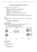
Multiplier diagram
Notes
Term 1
Lecture 1: Introduction to Demand Side
The Macroeconomy
Business cycle: Alternating periods of faster and slower (or even negative) growth rates. The
economy goes from boom to recession and back to boom.
Recessions:
o NBER definition: output is declining. A recession is over once the economy begins to grow
again.
o Alternative definition: the level of output is below its normal level, even if the economy is
growing. A recession is not over until output has grown enough to get back to normal.
it is a matter of judgement, and sometimes controversy, over what an economy’s
normal output would be
o During a recession unemployment increases which leads to a reduction in welfare
Measuring the economy
Aggregate output (GDP): The total output in an economy, across all sectors and regions.
o Three different ways of measuring GDP:
Spending: The total spent by households, firms, the government, and residents of other
countries on the home economy’s products.
Demand side – Y=C + I + G + (X-M)
Production: The total produced by the industries that operate in the home economy.
Production is measured by the value added by each industry: this means that the cost of
goods and services used as inputs to production is subtracted from the value of output.
These inputs will be measured in the value added of other industries, which prevents
double-counting when measuring production in the economy as a whole.
Y ≡ value of output sold — costs of raw materials and intermediate goods.
Income: The sum of all the incomes received, comprising wages, profits, the incomes of
the self-employed, and taxes received by the government.
Y≡ salaries of workers + profits of the owners of capital.
o While it can be defined according to any of these perspectives, globalisation means that it may
be occurring across different countries due to imports and exports
Therefore GDP includes exports and excludes imports
It is defined as the value added of domestic production, or as expenditure on domestic
production and as income due to domestic production
Consumption(c): Expenditure on consumer goods including both short-lived goods and services
and long-lived goods, which are called consumer durables.
o Largest component of GDP
o Less volatile due to consumption smoothing – there is certain spending that households
cannot put off e.g. food in a recession
Investment (I): Expenditure on newly produced capital goods (machinery and equipment) and
buildings, including new housing.
, o Investment in the unsold output that firms produce is called the change in inventories or stock
Inventory: Goods held by a firm prior to sale or use, including raw materials, and
partially-finished or finished goods intended for sale.
The purchase of a house is included in I, but all other consumption of durable goods
(cars, furniture) is included under consumption
o Represents a much lower share of GDP in OECD countries than in developing ones
o Much more volatile than other components of GDP as Firms do not face the same incentive to
smooth their expenditure as such spending can easily be postponed unlike spending on food
Firms increase their stock of machinery and equipment and build new premises
whenever they see an opportunity to make profits.
o This produces clusters of investment projects at some times
The boom following innovation occurs as all firms must switch to the new technology or
risk going out of business – they must install new machines
amplified if the firms producing the machinery and equipment need to expand
their own production facilities to meet the extra demand expected
Investment by one firm can also pull others to invest by helping to increase their market
and potential profits
Also can increase business confidence across the industry, resulting in bubbles
Credit constraints cause clustering as loans dry up during downturns and conversely in a
buoyant economy, profits are high and firms can use these profits to finance investment
projects.
Firms don’t invest when other firms aren’t investing even if they have low capacity
utilisation e.g. machinery and equipment are not being fully used.
The firm could produce more if it invested in hiring new workers but there isn’t
enough demand to sell those products and all other firms face the same
incentives not to invest
When both firms invest, the increase in employment leads to an increase in
consumption and thus demand, so profits of both would rise and they continue to
invest.
This is a virtuous circle, with both not investing and both investing being Nash
equilibria
Swings in business confidence act as a form of coordination between firms – one firm
develops optimistic beliefs about what another firm will do and thus invests
This has a major role in fluctuations of the economy as a whole.
Positive growth in demand leads to positive growth in investment – follows
fluctuations in national income more than consumption does
Government spending (G): Expenditure by the government to purchase goods and services.
When used as a component of aggregate demand, this does not include spending on transfers
such as pensions and unemployment benefits.
o Spending by the government in the form of payments to households or individuals.
Unemployment benefits and pensions are examples.
Exports (X): Goods and services produced in a particular country and sold to households, firms
and governments in other countries.
o trade balance value of exports minus the value of imports – net exports
Imports (M): Goods and services produced in other countries and purchased by domestic
households, firms, and the government.
, Aggregate demand: The total of the components of spending in the economy, added to get GDP:
Y = C + I + G + X – M. It is the total amount of demand for (or expenditure on) goods and services
produced in the economy
o GDP growth can be broken down into the contributions made by each component of
expenditure according to the share of GDP they account for
o Real expenditure on goods and services produced in the domestic economy
o What affects Aggregate demand?
Expectations about the future: firms decide to invest if future post-tax profits are
expected to be high. Consumers want to smooth their consumption over the
business cycle and their lifecycle.
Households may save as a precautionary measure if they expect incomes may
fall in the future or if there is a rise in uncertainty
The extent of credit constraints: these arise due the imperfect information faced by
lenders
Lenders require collateral to secure loans – usually property – which not all
consumers have
o Limiting their ability to consumption smooth
Changes in the value of collateral affect consumption and investment
The interest rate
Changes the cost of borrowing, thus affecting investment and making it
harder for households to consumption smooth
Also makes it more attractive to save money rather than spend it on
investment/consumption
o Investments must have higher rates of return for a firm to go
ahead with them under high interest rates
Creditor households would spend more under higher interest rates as their
incomes have risen
Models
Notation:
o Upper case letters: nominal
o Lower case letters: real
For example, 𝑤 = 𝑊/𝑃 means “the real wage is the nominal wage divided by the price
level”
o Interest rates always lower case:
𝜄 (“iota”) is the nominal interest rate
𝑟 the real interest rate
o Superscript e means expected
o Dynamic models need time (t) subscripts
The IS curve: shows the combinations of the interest rate and output at which aggregate
spending in the economy is equal to output.
, o Shows the demand side in a model – downwards sloping relationship
oAt high interest rates, demand is low as there is less spending on housing, consumer durables
and firm investment
Thus a low level of output is required to satisfy demand
A change in the interest rate is represented as a shift along the IS curve –
monetary policy
o The IS curve shifts when there is a change in profit or income growth expectations
Increased uncertainty results in a left shift – firms postpone investment so there
is lower investment spending at any interest rate
o Fiscal policy can shift the curve
E.g. in a recession (when IS curve has shifted to the left due to reduced profit
expectations) the government might launch a major expenditure plan and the IS
curve shifts right
At any given interest rate, the government is purchasing more goods
and services
Might also increase consumer/firm confidence
o It is assumed that suppliers will respond to higher demand and increase input or vice versa
o Fischer equation: r = i - Π e
The real interest rate is the nominal interest rate adjusted for expected inflation
We assume that all agents face the same real interest rate
Modelling the Goods Market Equilibrium
o Aggregate demand function:
yD = C + I + G
Equilibrium occurs where the planned real expenditure on goods and services
(AD) is equal to real output.
yD = y
o Aggregate consumption function:
C = C0 + C1(1-t)y
We assume that taxes are a fixed proportion of income
C1 is the MPC or fraction of income that is consumed – it shows the change in
consumption as the result of a change in post-tax/disposable income
Income is the amount that can be consumed without reducing your
assets
C0 is autonomous consumption
Multiplier diagram