Summary Transport & Economics and Management
Demand (lecture 1)
Why are we interested in demand? Understand consumer behaviour so we can develop
strategies to change the world (e.g. Apple). We derive demand by maximizing utility (fun).
What can we do with a demand function?
• Firms: estimate functions to predict demand
• Policy makers: determine welfare
• Willingness-to-pay: what does a customer want to pay?
Assumptions for demand function, the customer
is:
• Rational: you make the best decision
• Self-interested: making that decision
gives me a good feeling
• Maximizing utility
• Has a budget constraint:
At each point we have the combination of
𝑝1 𝑎𝑛𝑑 𝑄1 at which utility is maximized!
Reasonable assumptions? Yes, we are aware of
the limitations so the assumptions are quite
workable
Demand function: the customer makes a choice
on how much to buy of 𝑄1 or 𝑄2 given his/her
budget constraint. 𝑄 = 𝑎 − 𝑏 ∗ 𝑃
Views output as a function of price.
Budget constraint: 𝑌 = 𝑝1 𝑄1 + 𝑝2 𝑄2 Budget curve: 𝑄2 = (𝑌 − 𝑝1 ∗ 𝑄1 / 𝑝2 𝑄1 )
𝑝
• Slope budget curve: 𝑝1
2
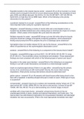
Indifference curve: combinations of 𝑄1 and 𝑄2 that yield the
same utility level. Indifference curve to the left means a lower
utility, to the right a higher utility. The indifference curve has
to meet the budget constraint (tangent) and at that point your
utility will be maximized for a given budget. If they not touch,
it’s not possible because it doesn’t fit in your budget.
∆𝑄
• Slope = ∆𝑄2
1
Amount of 𝑄2 we exchange for a unit of 𝑄1 , given level
of U
• Optimum:
slope budget curve=slope indifference curve
𝑝1 ∆𝑄
𝑝
= ∆𝑄2
2 1
Demand (lecture 1)
, 𝑎 1
Inverse demand: 𝑃 = 𝑏 − 𝑏 𝑄 (linear curve)
• Each point gives the combination of 𝑝1 and 𝑄1 at which
utility is maximized
• Maximum price we are willing to pay (value) so that our
utility is still maximized -> so gives willingness to pay.
• The (marginal) benefit we derive from 𝑄1 , often used as
measure of welfare -> so marginal benefit.
• Measures how much (value) of 𝑄2 is given up for more
𝑄1 , given that utility is maximized
• Views price as a function of output
𝑎
• 𝑏
𝑔𝑖𝑣𝑒𝑠 𝑡ℎ𝑒 ℎ𝑖𝑔ℎ𝑒𝑠𝑡 𝑤𝑖𝑙𝑙𝑖𝑛𝑔𝑛𝑒𝑠𝑠 𝑡𝑜 𝑝𝑎𝑦
1
• 𝑏
𝑔𝑖𝑣𝑒𝑠 ℎ𝑜𝑤 𝑡ℎ𝑒 𝑚𝑎𝑟𝑔𝑖𝑛𝑎𝑙 𝑏𝑒𝑛𝑒𝑓𝑖𝑡 𝑐ℎ𝑎𝑛𝑔𝑒𝑠 𝑤𝑖𝑡ℎ 𝑄
What determines demand?
• Price of substitutes
• Price of complementary goods
• Income changes
• Population
• Bureaucracy: more paperwork and administration cost time, which has a negative effect
on demand
• Popularity
• Speed: minimize time
• Reliability: appointments, just in time
• Security: security of transport
Elasticities
• % change in a variable as a result of 1% change in another variable.
• Arc elasticity: measures the effect of a substantial change in price.
o Demand function as a whole is elastic/inelastic (entire range of outputs)
• Point elasticity; measures elasticity at one specific point at the inverse demand function
(price change is very small)
• Why do we look at relative changes when we discuss elasticity?
o Most important: if you take absolute differences, you say increase the price with
2 dollar and demand decreases with 10000 products. -> difficult to compare
elasticities
o In order to be able compare between goods, previous years, markets.
Price elasticity of demand (point elasticity): responsiveness of demand to a change in price,
measured in percentages (because of different units, e.g. Q in tons, P in euros)
• % change in output / % change in price
∆𝑄 ∆𝑃 ∆𝑄 𝑄 𝜕𝑄 𝑃
• 𝑄 / 𝑃 = ( ∆𝑃 / 𝑃 ) -> 𝜕𝑃
∗ (𝑄 ) = partial derivative of Q with respect to P
• The price elasticity is not the slope of the demand curve
• E.g. price elasticity of -1.15 means that demand decreased by 1.15% if the price by 1%
increase
o Inelastic demand: −1 < 𝑝𝑟𝑖𝑐𝑒 𝑒𝑙𝑎𝑠𝑡𝑖𝑐𝑖𝑡𝑦 < 0
o Elastic demand: 𝑝𝑟𝑖𝑐𝑒 𝑒𝑙𝑎𝑠𝑡𝑖𝑐𝑖𝑡𝑦 < −1
Demand (lecture 1)
,Knowledge clip example:
𝑎 1
• 𝑃 =𝑏−𝑏∗𝑄 Linear inverse demand curve
• 𝑄 = 𝑎−𝑏∗𝑃 Rewrite of P
𝑎 𝑎
• If the output is then the elasticity is -1, because 𝑃𝑒𝑑 = −𝑏 ∗ 𝑎/(2𝑏)/( ) = −1.
2 2
• If the output is 0, then the elasticity is -infinite
• If the output is 𝑎 then is the elasticity always 0.
Price elasticity influenced by:
• Proportion of consumer expenditure: The smaller the proportion of total expenditure, the
more price inelastic it is likely to be. (bottle of water)
• Addictiveness: the more addictive, the more price inelastic. (cigarettes)
• Level of necessity: the greater the necessity, the more price inelastic. (bottle of water)
• Time scale: the longer the time period, the more price elastic. (substitutes)
• Availability of substitutes: the greater number of substitutes, the more elastic
Can price elasticity can be controlled?
• I can make my product look more necessary or make it more addictive
• But I am dependent on your behaviour as a reaction to my actions -> so not controllable.
Welfare: total benefit a consumer gets from buying a certain quantity at a certain price. The
(marginal) benefit consumers derive from additional good.
• Total benefit: area under inverse demand (up until point price equals 0)
• Welfare = total benefit (cs+pr) – total costs
Estimating demand
𝑄 = 𝑓(𝑃, 𝑌, 𝑡)
• Demand (Q) is a function of Price P, income Y and time trend t
• Q=α*P+β*Y+γ*t or lnQ=α*lnP+β*lnY+γ*t
o If you transform the variables into logarithms: the alpha automatically measures
elasticity
• It assumes a causal relation between variables (P, Y and t cause/explain Q)
Demand (lecture 1)
, Costs (lecture 2)
Cost function
• A cost function gives total costs as a function of output(s) and the prices of all inputs
o Gives the minimum cost of producing a given output level
• Choose production factors (land, labour, capital, entrepreneurship) so that costs are
minimized.
o Production output 𝑄 e.g. 𝑄 = 𝛿𝐿𝛼 𝐾𝛽
o Labour 𝐿 at price 𝑤
o Capital 𝐾 at price 𝑟
o 𝛼 𝑎𝑛𝑑 𝛽 are the weights of capital and labour in the production function
• Minimize: 𝐶 = 𝑤 ∗ 𝐿 + 𝑟 ∗ 𝐾
o Minimum cost of producing 𝑄 given input prices, using optimal levels of (𝐾, 𝐿)
• Application of cost function assumes cost minimization! (rational & self-interest)
o Reasonable? Yes, depending on which sector you are working (hospital)
Iso-cost: 𝐿 = (𝐶 − 𝑟 ∗ 𝐾)/𝑤
• Same idea as budget constraint for customers, how much labour can we buy?
𝑟
• Slope =
𝑤
Isoquant gives the amount of labour that we need,
given output target and amount of capital that we
have. Doesn’t matter where you are on the curve, it’s
the same output level.
1
• 𝐿 = 𝑄𝛿 −1 𝐾 −𝛽 ( 𝛼 )
∆𝐿
• 𝑆𝑙𝑜𝑝𝑒 =
∆𝐾
Cost minimization: the point where the isoquant and cost function meet each other
• slope iso-cost = slope isoquant
𝑟 ∆𝐿
=
𝑤 ∆𝐾
It depends on the price of labour and capital and the output level. Assumption of cost function:
output level is optimized (by required amount of labour and capital).
Cost function requirements:
• Cost increases with an output: you use more production factors so your Q will
increase. Q can never be minus. If you spend more, your output will never go down.
• Cost does not decrease with a price: if everything stays the same and the price
increases, your costs can never decrease.
• The prices of all inputs are included
• Changing to other currency will give same as changing every price to other dimension
o 𝐶(𝑄, 𝑥 ∗ 𝑤, 𝑥 ∗ 𝑟) = 𝑥 ∗ 𝐶(𝑄, 𝑤, 𝑟)
Three types of cost functions (not in ppt but handy to know):
• Cobb Douglas: functional form of a cost or production function that is linear in the logs. It
is estimated by using the method of least squares. Easy to estimate, mathematically
convenient and easier to interpret than translog. Downside that it is simplistic because it
assumes that firms have the same elasticities.
• Translog function: instead of begin linear in the logs, this function is quadratic in the
logs. More flexible form than Cobb Douglas, which results in less restrictions on the
elasticities. Downside: difficult to interpret and required more parameters.
• Linear function: linear in all the variables that are used.
Costs (lecture 2)
Demand (lecture 1)
Why are we interested in demand? Understand consumer behaviour so we can develop
strategies to change the world (e.g. Apple). We derive demand by maximizing utility (fun).
What can we do with a demand function?
• Firms: estimate functions to predict demand
• Policy makers: determine welfare
• Willingness-to-pay: what does a customer want to pay?
Assumptions for demand function, the customer
is:
• Rational: you make the best decision
• Self-interested: making that decision
gives me a good feeling
• Maximizing utility
• Has a budget constraint:
At each point we have the combination of
𝑝1 𝑎𝑛𝑑 𝑄1 at which utility is maximized!
Reasonable assumptions? Yes, we are aware of
the limitations so the assumptions are quite
workable
Demand function: the customer makes a choice
on how much to buy of 𝑄1 or 𝑄2 given his/her
budget constraint. 𝑄 = 𝑎 − 𝑏 ∗ 𝑃
Views output as a function of price.
Budget constraint: 𝑌 = 𝑝1 𝑄1 + 𝑝2 𝑄2 Budget curve: 𝑄2 = (𝑌 − 𝑝1 ∗ 𝑄1 / 𝑝2 𝑄1 )
𝑝
• Slope budget curve: 𝑝1
2
Indifference curve: combinations of 𝑄1 and 𝑄2 that yield the
same utility level. Indifference curve to the left means a lower
utility, to the right a higher utility. The indifference curve has
to meet the budget constraint (tangent) and at that point your
utility will be maximized for a given budget. If they not touch,
it’s not possible because it doesn’t fit in your budget.
∆𝑄
• Slope = ∆𝑄2
1
Amount of 𝑄2 we exchange for a unit of 𝑄1 , given level
of U
• Optimum:
slope budget curve=slope indifference curve
𝑝1 ∆𝑄
𝑝
= ∆𝑄2
2 1
Demand (lecture 1)
, 𝑎 1
Inverse demand: 𝑃 = 𝑏 − 𝑏 𝑄 (linear curve)
• Each point gives the combination of 𝑝1 and 𝑄1 at which
utility is maximized
• Maximum price we are willing to pay (value) so that our
utility is still maximized -> so gives willingness to pay.
• The (marginal) benefit we derive from 𝑄1 , often used as
measure of welfare -> so marginal benefit.
• Measures how much (value) of 𝑄2 is given up for more
𝑄1 , given that utility is maximized
• Views price as a function of output
𝑎
• 𝑏
𝑔𝑖𝑣𝑒𝑠 𝑡ℎ𝑒 ℎ𝑖𝑔ℎ𝑒𝑠𝑡 𝑤𝑖𝑙𝑙𝑖𝑛𝑔𝑛𝑒𝑠𝑠 𝑡𝑜 𝑝𝑎𝑦
1
• 𝑏
𝑔𝑖𝑣𝑒𝑠 ℎ𝑜𝑤 𝑡ℎ𝑒 𝑚𝑎𝑟𝑔𝑖𝑛𝑎𝑙 𝑏𝑒𝑛𝑒𝑓𝑖𝑡 𝑐ℎ𝑎𝑛𝑔𝑒𝑠 𝑤𝑖𝑡ℎ 𝑄
What determines demand?
• Price of substitutes
• Price of complementary goods
• Income changes
• Population
• Bureaucracy: more paperwork and administration cost time, which has a negative effect
on demand
• Popularity
• Speed: minimize time
• Reliability: appointments, just in time
• Security: security of transport
Elasticities
• % change in a variable as a result of 1% change in another variable.
• Arc elasticity: measures the effect of a substantial change in price.
o Demand function as a whole is elastic/inelastic (entire range of outputs)
• Point elasticity; measures elasticity at one specific point at the inverse demand function
(price change is very small)
• Why do we look at relative changes when we discuss elasticity?
o Most important: if you take absolute differences, you say increase the price with
2 dollar and demand decreases with 10000 products. -> difficult to compare
elasticities
o In order to be able compare between goods, previous years, markets.
Price elasticity of demand (point elasticity): responsiveness of demand to a change in price,
measured in percentages (because of different units, e.g. Q in tons, P in euros)
• % change in output / % change in price
∆𝑄 ∆𝑃 ∆𝑄 𝑄 𝜕𝑄 𝑃
• 𝑄 / 𝑃 = ( ∆𝑃 / 𝑃 ) -> 𝜕𝑃
∗ (𝑄 ) = partial derivative of Q with respect to P
• The price elasticity is not the slope of the demand curve
• E.g. price elasticity of -1.15 means that demand decreased by 1.15% if the price by 1%
increase
o Inelastic demand: −1 < 𝑝𝑟𝑖𝑐𝑒 𝑒𝑙𝑎𝑠𝑡𝑖𝑐𝑖𝑡𝑦 < 0
o Elastic demand: 𝑝𝑟𝑖𝑐𝑒 𝑒𝑙𝑎𝑠𝑡𝑖𝑐𝑖𝑡𝑦 < −1
Demand (lecture 1)
,Knowledge clip example:
𝑎 1
• 𝑃 =𝑏−𝑏∗𝑄 Linear inverse demand curve
• 𝑄 = 𝑎−𝑏∗𝑃 Rewrite of P
𝑎 𝑎
• If the output is then the elasticity is -1, because 𝑃𝑒𝑑 = −𝑏 ∗ 𝑎/(2𝑏)/( ) = −1.
2 2
• If the output is 0, then the elasticity is -infinite
• If the output is 𝑎 then is the elasticity always 0.
Price elasticity influenced by:
• Proportion of consumer expenditure: The smaller the proportion of total expenditure, the
more price inelastic it is likely to be. (bottle of water)
• Addictiveness: the more addictive, the more price inelastic. (cigarettes)
• Level of necessity: the greater the necessity, the more price inelastic. (bottle of water)
• Time scale: the longer the time period, the more price elastic. (substitutes)
• Availability of substitutes: the greater number of substitutes, the more elastic
Can price elasticity can be controlled?
• I can make my product look more necessary or make it more addictive
• But I am dependent on your behaviour as a reaction to my actions -> so not controllable.
Welfare: total benefit a consumer gets from buying a certain quantity at a certain price. The
(marginal) benefit consumers derive from additional good.
• Total benefit: area under inverse demand (up until point price equals 0)
• Welfare = total benefit (cs+pr) – total costs
Estimating demand
𝑄 = 𝑓(𝑃, 𝑌, 𝑡)
• Demand (Q) is a function of Price P, income Y and time trend t
• Q=α*P+β*Y+γ*t or lnQ=α*lnP+β*lnY+γ*t
o If you transform the variables into logarithms: the alpha automatically measures
elasticity
• It assumes a causal relation between variables (P, Y and t cause/explain Q)
Demand (lecture 1)
, Costs (lecture 2)
Cost function
• A cost function gives total costs as a function of output(s) and the prices of all inputs
o Gives the minimum cost of producing a given output level
• Choose production factors (land, labour, capital, entrepreneurship) so that costs are
minimized.
o Production output 𝑄 e.g. 𝑄 = 𝛿𝐿𝛼 𝐾𝛽
o Labour 𝐿 at price 𝑤
o Capital 𝐾 at price 𝑟
o 𝛼 𝑎𝑛𝑑 𝛽 are the weights of capital and labour in the production function
• Minimize: 𝐶 = 𝑤 ∗ 𝐿 + 𝑟 ∗ 𝐾
o Minimum cost of producing 𝑄 given input prices, using optimal levels of (𝐾, 𝐿)
• Application of cost function assumes cost minimization! (rational & self-interest)
o Reasonable? Yes, depending on which sector you are working (hospital)
Iso-cost: 𝐿 = (𝐶 − 𝑟 ∗ 𝐾)/𝑤
• Same idea as budget constraint for customers, how much labour can we buy?
𝑟
• Slope =
𝑤
Isoquant gives the amount of labour that we need,
given output target and amount of capital that we
have. Doesn’t matter where you are on the curve, it’s
the same output level.
1
• 𝐿 = 𝑄𝛿 −1 𝐾 −𝛽 ( 𝛼 )
∆𝐿
• 𝑆𝑙𝑜𝑝𝑒 =
∆𝐾
Cost minimization: the point where the isoquant and cost function meet each other
• slope iso-cost = slope isoquant
𝑟 ∆𝐿
=
𝑤 ∆𝐾
It depends on the price of labour and capital and the output level. Assumption of cost function:
output level is optimized (by required amount of labour and capital).
Cost function requirements:
• Cost increases with an output: you use more production factors so your Q will
increase. Q can never be minus. If you spend more, your output will never go down.
• Cost does not decrease with a price: if everything stays the same and the price
increases, your costs can never decrease.
• The prices of all inputs are included
• Changing to other currency will give same as changing every price to other dimension
o 𝐶(𝑄, 𝑥 ∗ 𝑤, 𝑥 ∗ 𝑟) = 𝑥 ∗ 𝐶(𝑄, 𝑤, 𝑟)
Three types of cost functions (not in ppt but handy to know):
• Cobb Douglas: functional form of a cost or production function that is linear in the logs. It
is estimated by using the method of least squares. Easy to estimate, mathematically
convenient and easier to interpret than translog. Downside that it is simplistic because it
assumes that firms have the same elasticities.
• Translog function: instead of begin linear in the logs, this function is quadratic in the
logs. More flexible form than Cobb Douglas, which results in less restrictions on the
elasticities. Downside: difficult to interpret and required more parameters.
• Linear function: linear in all the variables that are used.
Costs (lecture 2)