SUMMARY FMD LECTURES
FINANCIAL MODELLING AND DERIVATIVES
*PLEASE DON’T DISTRIBUTE
, Financial Modelling and Derivatives
Lecture 1
Introductory lecture, not relevant for the exam
Lecture 2
To calculate the return of a stock for a particular period of time:
Or in other words: Return = Dividend Yield + Capital Gains
For calculating the expected return, we simply multiply each return with its respective
probability, and we sum everything up E(R) = ∑ 𝑃𝑅 × 𝑅
Then we have the variance of the return Var (R) = ∑ 𝑃𝑅 × (𝑅 − 𝐸[𝑅])2
This also gives us the standard deviation (volatility), which is easier to interpret than the
variance, because it is in the same units as the returns SD (R) = √𝑉𝑎𝑟 (𝑅)
Because volatility is usually measured in % per annum, we have to annualize the volatility. If
we go from daily volatility to annual volatility σannual = σdaily x √252 (there are 252 trading
days).
We can use a security’s historical average return to estimate its actual expected return. To
calculate the historical average annual return, we have to sum up each annual return and then
1
divide it by the total number of years 𝑅̅ = ∑𝑇𝑡=1 𝑅𝑡 . It looks complicated, but it is just the
𝑇
calculation of the average, so if we look at 3 years and they have a return of 10%, 20% and
30%, the average annual return would be (10 + 20 + 30)/3 = 20%.
1
For the historical variance Var (R) = ∑𝑇𝑡=1(𝑅𝑡 − 𝑅̅)2
𝑇−1
Because the average return is just an estimate of the expected return, there will be some
𝑆𝐷 (𝑅)
estimation error, which is called standard error SE =
√𝑇
,When having calculated the standard error, one can make a confidence interval. In the case
of a 95% confidence interval Historical average return ± 1.96 * Standard error
If we look at a portfolio, we can calculate the weight for each investment by dividing the
𝑉𝑎𝑙𝑢𝑒 𝑖𝑛𝑣𝑒𝑠𝑡𝑚𝑒𝑛𝑡 𝑖
value of that investment by the total value of the portfolio 𝑥𝑖 = ,
𝑇𝑜𝑡𝑎𝑙 𝑣𝑎𝑙𝑢𝑒 𝑝𝑜𝑟𝑡𝑓𝑜𝑙𝑖𝑜
where x is the weight.
The return on portfolio is the weighted average of each investment in the portfolio. This is
calculated 𝑅𝑝 = ∑ 𝑥𝑖 𝑅𝑖 and for the expected return 𝐸[𝑅𝑝 ] = ∑ 𝑥𝑖 𝐸[𝑅𝑖 ]
The volatility of a portfolio is less than the volatility of individual stocks in that portfolio due
to diversification.
Finally, to find the risk of the portfolio, we must know the degree to which the assets’ returns
move together. We can measure this with the covariance and the correlation.
If the covariance is positive, the two returns tend to move together. If it’s negative, they tend
to move in opposite directions. The covariance can be calculated by doing the following:
𝐶𝑜𝑣(𝑅𝑖 , 𝑅𝑗 ) = 𝐸[(𝑅𝑖 − 𝐸[𝑅𝑖 ])(𝑅𝑗 − 𝐸[𝑅𝑗 ])]
For the historical covariance:
What the correlation tells us is by how much the stocks move together. Correlation does not
depend on their volatility and will be always between -1 and +1. To calculate correlation:
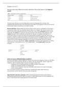
In a variance-covariance matrix like the one on the right, the diagonal
values going from up left to down right are the variances and the other
values are the covariances between both stocks. Because Cov (A, B) is
the same as Cov (B, A), they have both the same value (0.00055).
For the variance of a portfolio: Var (Rp) =
, Lecture 3
To calculate the variance of a large portfolio (this formula is easy to use if we use a variance-
covariance matrix):
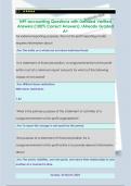
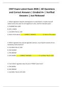
If we look at a variance-covariance matrix, we have
n variance terms and (n2 – n) covariance terms. For
example, this table has 4 variables (A, B, C, D),
therefore n = 4, n being the number of variables.
Because in a variance-covariance matrix, there are n
variance terms, we have in this case 4 variance terms (diagonal line). There are also 12
covariance terms, because (42 – 4) = 12.
With this in mind, we can simplify the formula of the variance of a large portfolio for an
equally weighted portfolio (same amount invested in each stock):
1 1
𝑉𝑎𝑟(𝑅𝑃 ) = (𝐴𝑣𝑒𝑟𝑎𝑔𝑒 𝑉𝑎𝑟𝑖𝑎𝑛𝑐𝑒 𝑜𝑓 𝐼𝑛𝑑𝑖𝑣𝑖𝑑𝑢𝑎𝑙 𝑠𝑡𝑜𝑐𝑘𝑠) + (1 − ) (𝐴𝑣𝑒𝑟𝑎𝑔𝑒 𝐶𝑜𝑣𝑎𝑟𝑖𝑎𝑛𝑐𝑒 𝑏𝑒𝑡𝑤𝑒𝑒𝑛 𝑡ℎ𝑒 𝑠𝑡𝑜𝑐𝑘𝑠)
𝑛 𝑛
As n increases, the variances of individual stocks
have less and less importance on determining the
total variance of the portfolio (because 1/n
decreases). Also, when n increases, the average
covariance between the stocks becomes more
important in determining the total variance. This
means that as you add more stocks, the
individual risks become less important, but the
correlated risk becomes more important.
To calculate the standard deviation of a portfolio with arbitrary weights:
FINANCIAL MODELLING AND DERIVATIVES
*PLEASE DON’T DISTRIBUTE
, Financial Modelling and Derivatives
Lecture 1
Introductory lecture, not relevant for the exam
Lecture 2
To calculate the return of a stock for a particular period of time:
Or in other words: Return = Dividend Yield + Capital Gains
For calculating the expected return, we simply multiply each return with its respective
probability, and we sum everything up E(R) = ∑ 𝑃𝑅 × 𝑅
Then we have the variance of the return Var (R) = ∑ 𝑃𝑅 × (𝑅 − 𝐸[𝑅])2
This also gives us the standard deviation (volatility), which is easier to interpret than the
variance, because it is in the same units as the returns SD (R) = √𝑉𝑎𝑟 (𝑅)
Because volatility is usually measured in % per annum, we have to annualize the volatility. If
we go from daily volatility to annual volatility σannual = σdaily x √252 (there are 252 trading
days).
We can use a security’s historical average return to estimate its actual expected return. To
calculate the historical average annual return, we have to sum up each annual return and then
1
divide it by the total number of years 𝑅̅ = ∑𝑇𝑡=1 𝑅𝑡 . It looks complicated, but it is just the
𝑇
calculation of the average, so if we look at 3 years and they have a return of 10%, 20% and
30%, the average annual return would be (10 + 20 + 30)/3 = 20%.
1
For the historical variance Var (R) = ∑𝑇𝑡=1(𝑅𝑡 − 𝑅̅)2
𝑇−1
Because the average return is just an estimate of the expected return, there will be some
𝑆𝐷 (𝑅)
estimation error, which is called standard error SE =
√𝑇
,When having calculated the standard error, one can make a confidence interval. In the case
of a 95% confidence interval Historical average return ± 1.96 * Standard error
If we look at a portfolio, we can calculate the weight for each investment by dividing the
𝑉𝑎𝑙𝑢𝑒 𝑖𝑛𝑣𝑒𝑠𝑡𝑚𝑒𝑛𝑡 𝑖
value of that investment by the total value of the portfolio 𝑥𝑖 = ,
𝑇𝑜𝑡𝑎𝑙 𝑣𝑎𝑙𝑢𝑒 𝑝𝑜𝑟𝑡𝑓𝑜𝑙𝑖𝑜
where x is the weight.
The return on portfolio is the weighted average of each investment in the portfolio. This is
calculated 𝑅𝑝 = ∑ 𝑥𝑖 𝑅𝑖 and for the expected return 𝐸[𝑅𝑝 ] = ∑ 𝑥𝑖 𝐸[𝑅𝑖 ]
The volatility of a portfolio is less than the volatility of individual stocks in that portfolio due
to diversification.
Finally, to find the risk of the portfolio, we must know the degree to which the assets’ returns
move together. We can measure this with the covariance and the correlation.
If the covariance is positive, the two returns tend to move together. If it’s negative, they tend
to move in opposite directions. The covariance can be calculated by doing the following:
𝐶𝑜𝑣(𝑅𝑖 , 𝑅𝑗 ) = 𝐸[(𝑅𝑖 − 𝐸[𝑅𝑖 ])(𝑅𝑗 − 𝐸[𝑅𝑗 ])]
For the historical covariance:
What the correlation tells us is by how much the stocks move together. Correlation does not
depend on their volatility and will be always between -1 and +1. To calculate correlation:
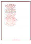
In a variance-covariance matrix like the one on the right, the diagonal
values going from up left to down right are the variances and the other
values are the covariances between both stocks. Because Cov (A, B) is
the same as Cov (B, A), they have both the same value (0.00055).
For the variance of a portfolio: Var (Rp) =
, Lecture 3
To calculate the variance of a large portfolio (this formula is easy to use if we use a variance-
covariance matrix):
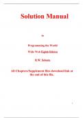
If we look at a variance-covariance matrix, we have
n variance terms and (n2 – n) covariance terms. For
example, this table has 4 variables (A, B, C, D),
therefore n = 4, n being the number of variables.
Because in a variance-covariance matrix, there are n
variance terms, we have in this case 4 variance terms (diagonal line). There are also 12
covariance terms, because (42 – 4) = 12.
With this in mind, we can simplify the formula of the variance of a large portfolio for an
equally weighted portfolio (same amount invested in each stock):
1 1
𝑉𝑎𝑟(𝑅𝑃 ) = (𝐴𝑣𝑒𝑟𝑎𝑔𝑒 𝑉𝑎𝑟𝑖𝑎𝑛𝑐𝑒 𝑜𝑓 𝐼𝑛𝑑𝑖𝑣𝑖𝑑𝑢𝑎𝑙 𝑠𝑡𝑜𝑐𝑘𝑠) + (1 − ) (𝐴𝑣𝑒𝑟𝑎𝑔𝑒 𝐶𝑜𝑣𝑎𝑟𝑖𝑎𝑛𝑐𝑒 𝑏𝑒𝑡𝑤𝑒𝑒𝑛 𝑡ℎ𝑒 𝑠𝑡𝑜𝑐𝑘𝑠)
𝑛 𝑛
As n increases, the variances of individual stocks
have less and less importance on determining the
total variance of the portfolio (because 1/n
decreases). Also, when n increases, the average
covariance between the stocks becomes more
important in determining the total variance. This
means that as you add more stocks, the
individual risks become less important, but the
correlated risk becomes more important.
To calculate the standard deviation of a portfolio with arbitrary weights: