Probability models
Inferential statistics related a given sample to a population by creating inferences. This is done by
Pr (data∨H 0 ) the probability of the data sample given that the H0 is true.
Empirical- distribution from a sample
Theoretical- precited when we look at a population and point out all the outcomes.
Expected value= avg outcome of random event X
E(X)→μ
Pr ( Xi)× Xi
E ( X ) =∑ →(nπ )
n
Variance= measure of the dispersion of the outcomes
var ( X ) → σ 2
var ( X )=∑ ¿ ¿ ¿
A random variable can be composed from multiple random variables. Two random variables can be
combined to form a single random variable. For the variance the following rule applies:
var ( A+ B )=var ( A−B )=var ( A )+ var ( B )
This rule is applicable as long as A and B are independent random variables.
Probability function
Probability always between 0 1
The sum is always 1 and the exact probability can be calculated.
Either binomial: dichotomous variable of poisons: discrete variable
Binomial distribution
Dichotomous variable
Success=1 Pr ( success )=π
No success=0 Pr ( no success ) =1−π
n! k
Pr ( X=k )= π ¿
k ! ( n−k ) !
Assumption: repeated trials are assumed to be independent. If it were dependent, then the probability
would change each successive time making it a non-binomial distribution.
Poisson
Discrete (finite) variables during a fixed time period or space
The distribution of a given number of independent counts 1 count does not rely on the previous count
−λ k
e λ
Pr ( X=k )=
k!
K is the number of events
γ is the expected value in this case E ( X ) =var ( X )
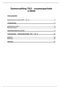
, Skewness
Right skew to the left of the graph making it negative
- Usually when π is low
Left skew to the right of the graph making it positive
- Usually when π is high
- Usually when γ is low
When π=0.5 there is an even distribution but also when n
increases. Also, when γ increases the distribution
becomes more symmetrical
Probability density function
Probability can range from 0 ∞
The area under the curve is 1 and the probability is estimated by the area
Either normal distribution: continuous or standard normal.
Normal distribution
Continuous variable
Theoretical probability also possible for discrete variables
Described by a normal density curve
****rarely done manually
Rule of thumb:
Pr ( X ≤ n ) =1−Pr ( X > n)
Where:
X N (μ , σ )
σ is small then the distribution is narrow
σ is larger then the distribution is more extended/broad
The peak depends on μ= E ( X )
Both E(X) and var(X) are critical characteristics
Standard normal distribution
Is the transformed normal distribution with:
μ=0∧σ=1
Only works on normal distribution- if they are skewed to the right sometimes the log-model is applied
which changes the distribution to look more normal.
Do this by calculating the z-score
X−μ
Z=
σ
With the z-score you check the probability in the table
Central limit theorem
As n increases the point estimate becomes narrower and more symmetrical normal distribution. Also, it
will no longer match the theoretical probability model
Inferential statistics related a given sample to a population by creating inferences. This is done by
Pr (data∨H 0 ) the probability of the data sample given that the H0 is true.
Empirical- distribution from a sample
Theoretical- precited when we look at a population and point out all the outcomes.
Expected value= avg outcome of random event X
E(X)→μ
Pr ( Xi)× Xi
E ( X ) =∑ →(nπ )
n
Variance= measure of the dispersion of the outcomes
var ( X ) → σ 2
var ( X )=∑ ¿ ¿ ¿
A random variable can be composed from multiple random variables. Two random variables can be
combined to form a single random variable. For the variance the following rule applies:
var ( A+ B )=var ( A−B )=var ( A )+ var ( B )
This rule is applicable as long as A and B are independent random variables.
Probability function
Probability always between 0 1
The sum is always 1 and the exact probability can be calculated.
Either binomial: dichotomous variable of poisons: discrete variable
Binomial distribution
Dichotomous variable
Success=1 Pr ( success )=π
No success=0 Pr ( no success ) =1−π
n! k
Pr ( X=k )= π ¿
k ! ( n−k ) !
Assumption: repeated trials are assumed to be independent. If it were dependent, then the probability
would change each successive time making it a non-binomial distribution.
Poisson
Discrete (finite) variables during a fixed time period or space
The distribution of a given number of independent counts 1 count does not rely on the previous count
−λ k
e λ
Pr ( X=k )=
k!
K is the number of events
γ is the expected value in this case E ( X ) =var ( X )
, Skewness
Right skew to the left of the graph making it negative
- Usually when π is low
Left skew to the right of the graph making it positive
- Usually when π is high
- Usually when γ is low
When π=0.5 there is an even distribution but also when n
increases. Also, when γ increases the distribution
becomes more symmetrical
Probability density function
Probability can range from 0 ∞
The area under the curve is 1 and the probability is estimated by the area
Either normal distribution: continuous or standard normal.
Normal distribution
Continuous variable
Theoretical probability also possible for discrete variables
Described by a normal density curve
****rarely done manually
Rule of thumb:
Pr ( X ≤ n ) =1−Pr ( X > n)
Where:
X N (μ , σ )
σ is small then the distribution is narrow
σ is larger then the distribution is more extended/broad
The peak depends on μ= E ( X )
Both E(X) and var(X) are critical characteristics
Standard normal distribution
Is the transformed normal distribution with:
μ=0∧σ=1
Only works on normal distribution- if they are skewed to the right sometimes the log-model is applied
which changes the distribution to look more normal.
Do this by calculating the z-score
X−μ
Z=
σ
With the z-score you check the probability in the table
Central limit theorem
As n increases the point estimate becomes narrower and more symmetrical normal distribution. Also, it
will no longer match the theoretical probability model