ORL - Decision Science
Lecture 1 - 30-8
1.Linear programming
Decision variables
Xa = # product A
Xb = # product B
Type Demand Capacity Profit
A 4 A+B = 6 2
B 3 A+B = 6 5
W = 2Xa + 5Xb
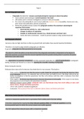
Set of constraints:
1) Xa ≤ 4 feasible area
2) Xb ≤ 3
3) Xa + Xb ≤ 6
Non-negativity constraint: Xa, Xb ≥ 0
Constraints
Xa = 0, Xb = 6 → (0,6). Xb = 0, Xa = 6 → (6,0)
Gradient: look at the w = 2Xa + 5Xb → 2 units to the right, 5 units up (red line from the origin) (direction
vector) (all points on this line have the same objective function value)
Isoquant: line perpendicular to the gradient.
𝑋𝑎 3
Unique optimal solution: = (3,3) → ( 𝑋𝑏 ) = ( 3 ) → 2*3 + 5*3 = 21
Binding vs Non-Binding
Binding = (2) Xb ≤ 3,(3) Xa + Xb ≤ 6
Non-binding = (1) Xa ≤ 4 will never affect the optimal solution
How can you see if a constraint is binding? →
1. Change the constraints in equality constraints (associate the slack with a new variable ‘y’):
(1)Xa ≤ 4 → Xa + Y1 = 4
(2)Xb ≤ 3 → Xb + Y2 = 3
(3)Xa + Xb ≤ 6 → Xa + Xb + Y3 = 6
2. Fill the coordinates from the optimal solution in the formulas and find Y:
(1) 3 + Y1 = 4 → Y1 = 1 → non-binding
(2) 3 + Y2 = 3 → Y2 = 0 → binding
(3) 3 + 3 + Y3 = 6 → Y3 = 0 → binding
,If the slack variable is positive, then the corresponding constraint is non-binding. SLACK=NON-BINDING
If the slack variable is equal to 0, then the corresponding constraint is binding.
NO SLACK=BINDING
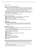
2. Linear programming with multiple solutions
Max ❵ 2X1 + 2X2
St.
(1) X1 ≤ 4
(2) X2 ≤ 3
(3) X1 + X2 ≤ 6
X1 + X2 ≥ 0
Gradient is parallel to the 3th constraint
Multiple solutions → line segment of alt. opt. sol. (you can describe this with a parameter equation)
3. Another kind of linear programming
Max ❵ w= -3X1 + 3X2
St.
(1) X1 + X2 ≥ 3
(2) -X1 + X2 ≤ 1
X1 + X2 ≥ 0
The relations between the variables are linear
Halfline of alt. opt. sol. (there are lots of solutions)
4. Maximization problem
W = 2X1 + 5X2
St.
(1) X1 + X2 ≥ 3
(2) -X1 + X2 ≤ 1
X1 + X2 ≥ 0
,Unbounded problem: you will never hit another point on the line (2) → you can always increase the
objective. You will never hit the ultimate dot.
5. Maximization problem
W = 2X1 + 5X2
St.
(1) X1 ≥ 4
(2) X1 + X2 ≤ 3
X1 + X2 ≥ 0
Infeasible problem: you can’t be in the two feasible areas at the same time.
Lecture 2 1-9-2021
Maximisation problem
Max ❴ W ≤ c’ x ❵
St A x ≤ b
x≥0
Sensitivity analysis:
1. Objective function
w = 2x1 + 5x2
st
(1) X1 ≤ 4
(2) X2 ≤ 3
(3) X1 + X2 ≤ 6
, Now replace the 2 for a parameter → ⍺ → make a table
There are multiple optimal options when you use the parameter ⍺ → line segment of alternative optimal
solutions → when ⍺ is lower or equal to 0, you always find the same optimal solution.
⍺ Optimal X* W*=⍺X1+5X2
(1) ⍺ ≤ 0 𝑋1
( 𝑋2 ) = ( 3 )
0 W* = 15
(2) 0 ≤ ⍺ ≤ 5 (3)
3 W* = 3⍺ + 15
(3) 5 ≤ ⍺ (2)
4 W* = 4⍺ + 10
The value 5 for X1 gives you the equation 5x1 + 5x2, which gives you a gradient perpendicular to the
third constraint of X1 + X2 ≤ 6. That is how you know that up till the value of 5, the optimal solution can be
found in the orange dot in the graph above.
Pacewise linear curve. Parametric programming:
2. The right-hand side (RHS)
Is it worthwhile to put money in extra labour or advertisement, if you make additional costs, will you get it
out?
Now we will use parameter 𝛃;
Max ❴ W = 2X1 + 5X2 ❵
St
(1) X1 ≤ 4
(2) X2 ≤ 𝛃
(3) X1 + X2 ≤ 6
𝛃 X* W
-infinity ≤ 𝛃 ≤ 0 infeasible infeasible
0≤𝛃≤2 𝑋1 4
( 𝑋2 )* = ( 𝛃 ) w*= 8+ 5𝛃
2≤𝛃≤6 𝑋1
( 𝑋2 )* = (
6−𝛃
) w*=2(6-𝛃)+5𝛃
𝛃
𝛃≥6 𝑋1 0
( 𝑋2 )* = ( 6 ) w* = 30
Lecture 1 - 30-8
1.Linear programming
Decision variables
Xa = # product A
Xb = # product B
Type Demand Capacity Profit
A 4 A+B = 6 2
B 3 A+B = 6 5
W = 2Xa + 5Xb
Set of constraints:
1) Xa ≤ 4 feasible area
2) Xb ≤ 3
3) Xa + Xb ≤ 6
Non-negativity constraint: Xa, Xb ≥ 0
Constraints
Xa = 0, Xb = 6 → (0,6). Xb = 0, Xa = 6 → (6,0)
Gradient: look at the w = 2Xa + 5Xb → 2 units to the right, 5 units up (red line from the origin) (direction
vector) (all points on this line have the same objective function value)
Isoquant: line perpendicular to the gradient.
𝑋𝑎 3
Unique optimal solution: = (3,3) → ( 𝑋𝑏 ) = ( 3 ) → 2*3 + 5*3 = 21
Binding vs Non-Binding
Binding = (2) Xb ≤ 3,(3) Xa + Xb ≤ 6
Non-binding = (1) Xa ≤ 4 will never affect the optimal solution
How can you see if a constraint is binding? →
1. Change the constraints in equality constraints (associate the slack with a new variable ‘y’):
(1)Xa ≤ 4 → Xa + Y1 = 4
(2)Xb ≤ 3 → Xb + Y2 = 3
(3)Xa + Xb ≤ 6 → Xa + Xb + Y3 = 6
2. Fill the coordinates from the optimal solution in the formulas and find Y:
(1) 3 + Y1 = 4 → Y1 = 1 → non-binding
(2) 3 + Y2 = 3 → Y2 = 0 → binding
(3) 3 + 3 + Y3 = 6 → Y3 = 0 → binding
,If the slack variable is positive, then the corresponding constraint is non-binding. SLACK=NON-BINDING
If the slack variable is equal to 0, then the corresponding constraint is binding.
NO SLACK=BINDING
2. Linear programming with multiple solutions
Max ❵ 2X1 + 2X2
St.
(1) X1 ≤ 4
(2) X2 ≤ 3
(3) X1 + X2 ≤ 6
X1 + X2 ≥ 0
Gradient is parallel to the 3th constraint
Multiple solutions → line segment of alt. opt. sol. (you can describe this with a parameter equation)
3. Another kind of linear programming
Max ❵ w= -3X1 + 3X2
St.
(1) X1 + X2 ≥ 3
(2) -X1 + X2 ≤ 1
X1 + X2 ≥ 0
The relations between the variables are linear
Halfline of alt. opt. sol. (there are lots of solutions)
4. Maximization problem
W = 2X1 + 5X2
St.
(1) X1 + X2 ≥ 3
(2) -X1 + X2 ≤ 1
X1 + X2 ≥ 0
,Unbounded problem: you will never hit another point on the line (2) → you can always increase the
objective. You will never hit the ultimate dot.
5. Maximization problem
W = 2X1 + 5X2
St.
(1) X1 ≥ 4
(2) X1 + X2 ≤ 3
X1 + X2 ≥ 0
Infeasible problem: you can’t be in the two feasible areas at the same time.
Lecture 2 1-9-2021
Maximisation problem
Max ❴ W ≤ c’ x ❵
St A x ≤ b
x≥0
Sensitivity analysis:
1. Objective function
w = 2x1 + 5x2
st
(1) X1 ≤ 4
(2) X2 ≤ 3
(3) X1 + X2 ≤ 6
, Now replace the 2 for a parameter → ⍺ → make a table
There are multiple optimal options when you use the parameter ⍺ → line segment of alternative optimal
solutions → when ⍺ is lower or equal to 0, you always find the same optimal solution.
⍺ Optimal X* W*=⍺X1+5X2
(1) ⍺ ≤ 0 𝑋1
( 𝑋2 ) = ( 3 )
0 W* = 15
(2) 0 ≤ ⍺ ≤ 5 (3)
3 W* = 3⍺ + 15
(3) 5 ≤ ⍺ (2)
4 W* = 4⍺ + 10
The value 5 for X1 gives you the equation 5x1 + 5x2, which gives you a gradient perpendicular to the
third constraint of X1 + X2 ≤ 6. That is how you know that up till the value of 5, the optimal solution can be
found in the orange dot in the graph above.
Pacewise linear curve. Parametric programming:
2. The right-hand side (RHS)
Is it worthwhile to put money in extra labour or advertisement, if you make additional costs, will you get it
out?
Now we will use parameter 𝛃;
Max ❴ W = 2X1 + 5X2 ❵
St
(1) X1 ≤ 4
(2) X2 ≤ 𝛃
(3) X1 + X2 ≤ 6
𝛃 X* W
-infinity ≤ 𝛃 ≤ 0 infeasible infeasible
0≤𝛃≤2 𝑋1 4
( 𝑋2 )* = ( 𝛃 ) w*= 8+ 5𝛃
2≤𝛃≤6 𝑋1
( 𝑋2 )* = (
6−𝛃
) w*=2(6-𝛃)+5𝛃
𝛃
𝛃≥6 𝑋1 0
( 𝑋2 )* = ( 6 ) w* = 30