Lectures Transport economics and management
Lecture 1
Introduction Demand analysis
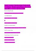
Golden circle (simon sinek)
What makes a great leader, a great leader is a person that
starts with the question: Why? Then you can know : how
should i do this? Than you can know what you have to do. So
it starts with motivation. Then you go to procedures and
methods, which will lead to products and services.
There are leaders and followers in the model. A good
example is Apple. Why: the want to change the world. How:
good design. What: and one more thing?
- Policy maker: leader
• Why: Change the world
• How: improve society and position of inhabitants
• What: whatever policy is necessary
* Is why to what
- Policy maker: follower
• Why: “Because we read about it in the newspaper”
• How: improve society and position of inhabitants
• What: take action (policy)
* Is what to why
- Manager: leader
• Why: Incentives
• How: I design an optimal process
• What: I deliver a product/service
* is from why to what
- Manager: follower
• Why: Because I have to
• How: using some process
• What: I deliver a product/service
* is from what to why
EU Transport policy
• EU transport policy
> EC aims to develop and promote transport policies that are efficient, safe, secure and sustainable,
to create the conditions for a competitive industry that generates jobs and prosperity.
> Inspiration (Why?): prosperity
> Method (how?): competitive industry (amongst other things)
> What: Policy
• This will have an effect on your company
• Understand policy background
• Understand incentives and consumer/producer behavior
1
,Demand
The economics of demand
- Why are we interested in demand? -> to understand consumer behaviour. You can develop
strategies to change the world. Why do consumers behave like this
- How do we derive demand?
> Maximize utility; “inverse demand”
> Assumptions: rational and self-interested consumers, utility maximization
> Reasonable assumptions? To some extent yes, it is a model or a simplification of reality. It is a
model of how a representative consumer would behave. The conditions are not always met, but the
model assumes it is to be able to calculate.
What can we do with a demand function?
> Firms: estimate demand functions (e.g. OLS) to predict demand
> Policy maker: determine welfare
> Willingness-to-pay: what does the client want to pay?
What determines demand
There are multiple factors determining the height of the inverse demand
function
• Price of substitutes • Price of complementary goods • Income •
Population • Bureaucracy • Security • Popularity/image • Speed • Reliability
- Which factors are relevant for you as manager? Speed, reliability, price of substitutes, security.
- Which factors are controllable for you as manager? speed, reliability, security, image, sometimes
price of complementary goods but that has far reaching consequences for the company. no factor is
100% controllable, you are always depended on other factors and
the environment.
KENNISCLIP INVERSE DEMAND
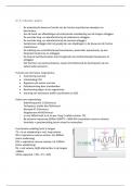
- assumptions about the consumer: -> is rational, self- interested
and wants to maximize utility U.
- consumer makes a choice on how much to buy of goods Q1 and
Q2 given the consumer’s budget constraint Y= P1*Q1 + P2*Q2
Indifference curve: combinations of Q1 and Q2 that yield the same utility level
- the formula can be rewritten as Q2= (Y- P1*Q1) / P2, which gives a budget curve.
if we spend nothing on Q1, the total budget goes to Q2 (left top)
is budget/ P2. If we give up some of Q2 to get Q1, we move over
the budget line.
- Slope of the curve= -p1/ p2
The indifference curve: the higher the curve, the higher the level
of utility. The slope of the curve tells how much you need to
give up from Q2 to be able to get Q1, given a certain level of
utility.
the indifference curve has a technical requirement. The convex needs to go to the origin: A and B are
two points on the curve a ray passing through O and D meets the indifference curve at one point (C)
between O and D. implication is that indifference curve do not intersect!
2
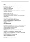
,the optimal combination of Q1 and Q2 (max utility) is at the point where the slope of the budget
curve= slope highest possible indifference curve.
Example
given Y P1 and P2 we have the optimum show. The right side is the same P1 and Q1. If we reduce P1,
the slope becomes less steep (black line), which gives a new
optimum. This is also represented in the right graph. If P1 is
reduced even further, the budget constraint will be more
shallow (golden line).
If we combine the corner points, you get the inverse demand
function. This gives the relation between P1 and Q1, the price
that can be charged so that utility is maximized. This can be
seen from the left slide.
Linear inverse demand curve are used for simplicity. P= a/b – 1/b *Q
Interpretation of (inverse) demand curve:
- in the optimum (D ) : slope budget curve= slope indifference curve -> p1/p2 = delta Q2/ delta Q1
- at the margin: extra room in budget created by reducing Q2= extra room needed to get more Q1:
P1* deltaQ1= p2 *delta Q2
- Inverse demand: P1=p2* delta Q2/ delta Q1
- maximum price we are willing to pay (and a company can charge so that our utility is still maximized
- the benefit (surplus) we derive from Q1 (Expressed in monetary terms): often used as measure of
welfare (as used in cost-benefit- analysis
- measures how much (value) of Q2 is given up for more Q1, given that utility is maximized
3
, Elasticities
Is the % change in a variable as a result of a % change in another variable
> Arc vs point elasticity
arc means if we look at the price elasticity in demand we look at the change in demand.
- point is if we have inverse demand function, we pick a point and change the price a little bit.
> Why relative changes?
- Because it depends on the base, you want to see it in perspective. A price change of 5 for example
does not say anything about the base, so if you start with low or high output levels. You are looking
for relationships between variables, therefore you need a solid base. It is the height of the price in
relation to the output level.
Determinants of elasticities
- Price elasticity of demand is the change of demand because of a change in the price.
- Price elasticity is influenced by:
> proportion of consumer expenditure (what do I have to give up to get the new Iphone)
> addictiveness (people who are addicted are less sensitive for the price).
> level of necessity (if the price of water is high people still buy it because you need to have drinks)
> time scale
> availability of substitutes
Can an elasticity be “controlled”?
- a price elasticity reflects consumer preferences. The price or opinions can be changed, but not
specifically the elasticity. So no.
Welfare
Consumers
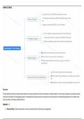
> inverse demand curve gives willingness- to-pay.
> Benefit consumer(s) derive(s) from additional good
> marginal benefit: the value of everything else I need to give up
to get the product.
> area under inverse demand curve measures total benefit or total
surplus. Value everyone is willing to give up to get all the units up
to a certain point.
- if there is a supply function, the equilibrium is at the intersection.
the price is pe and demand is Qe. The total surplus is from 0 to Q1
up to P.
Estimating demand
• Q=f(P, Y, t)
> Demand (Q) is a function of price P, income Y and time
trend t.
> Q=α*P+β*Y+γ*t or lnQ=α*lnP+β*lnY+γ*t
• Assumes a causal relation between variables
> P, Y and t‘ cause’ Q
> data on prices, demand, income and other
characteristics needed
• Part of tutorial > time series > OLS
4
Lecture 1
Introduction Demand analysis
Golden circle (simon sinek)
What makes a great leader, a great leader is a person that
starts with the question: Why? Then you can know : how
should i do this? Than you can know what you have to do. So
it starts with motivation. Then you go to procedures and
methods, which will lead to products and services.
There are leaders and followers in the model. A good
example is Apple. Why: the want to change the world. How:
good design. What: and one more thing?
- Policy maker: leader
• Why: Change the world
• How: improve society and position of inhabitants
• What: whatever policy is necessary
* Is why to what
- Policy maker: follower
• Why: “Because we read about it in the newspaper”
• How: improve society and position of inhabitants
• What: take action (policy)
* Is what to why
- Manager: leader
• Why: Incentives
• How: I design an optimal process
• What: I deliver a product/service
* is from why to what
- Manager: follower
• Why: Because I have to
• How: using some process
• What: I deliver a product/service
* is from what to why
EU Transport policy
• EU transport policy
> EC aims to develop and promote transport policies that are efficient, safe, secure and sustainable,
to create the conditions for a competitive industry that generates jobs and prosperity.
> Inspiration (Why?): prosperity
> Method (how?): competitive industry (amongst other things)
> What: Policy
• This will have an effect on your company
• Understand policy background
• Understand incentives and consumer/producer behavior
1
,Demand
The economics of demand
- Why are we interested in demand? -> to understand consumer behaviour. You can develop
strategies to change the world. Why do consumers behave like this
- How do we derive demand?
> Maximize utility; “inverse demand”
> Assumptions: rational and self-interested consumers, utility maximization
> Reasonable assumptions? To some extent yes, it is a model or a simplification of reality. It is a
model of how a representative consumer would behave. The conditions are not always met, but the
model assumes it is to be able to calculate.
What can we do with a demand function?
> Firms: estimate demand functions (e.g. OLS) to predict demand
> Policy maker: determine welfare
> Willingness-to-pay: what does the client want to pay?
What determines demand
There are multiple factors determining the height of the inverse demand
function
• Price of substitutes • Price of complementary goods • Income •
Population • Bureaucracy • Security • Popularity/image • Speed • Reliability
- Which factors are relevant for you as manager? Speed, reliability, price of substitutes, security.
- Which factors are controllable for you as manager? speed, reliability, security, image, sometimes
price of complementary goods but that has far reaching consequences for the company. no factor is
100% controllable, you are always depended on other factors and
the environment.
KENNISCLIP INVERSE DEMAND
- assumptions about the consumer: -> is rational, self- interested
and wants to maximize utility U.
- consumer makes a choice on how much to buy of goods Q1 and
Q2 given the consumer’s budget constraint Y= P1*Q1 + P2*Q2
Indifference curve: combinations of Q1 and Q2 that yield the same utility level
- the formula can be rewritten as Q2= (Y- P1*Q1) / P2, which gives a budget curve.
if we spend nothing on Q1, the total budget goes to Q2 (left top)
is budget/ P2. If we give up some of Q2 to get Q1, we move over
the budget line.
- Slope of the curve= -p1/ p2
The indifference curve: the higher the curve, the higher the level
of utility. The slope of the curve tells how much you need to
give up from Q2 to be able to get Q1, given a certain level of
utility.
the indifference curve has a technical requirement. The convex needs to go to the origin: A and B are
two points on the curve a ray passing through O and D meets the indifference curve at one point (C)
between O and D. implication is that indifference curve do not intersect!
2
,the optimal combination of Q1 and Q2 (max utility) is at the point where the slope of the budget
curve= slope highest possible indifference curve.
Example
given Y P1 and P2 we have the optimum show. The right side is the same P1 and Q1. If we reduce P1,
the slope becomes less steep (black line), which gives a new
optimum. This is also represented in the right graph. If P1 is
reduced even further, the budget constraint will be more
shallow (golden line).
If we combine the corner points, you get the inverse demand
function. This gives the relation between P1 and Q1, the price
that can be charged so that utility is maximized. This can be
seen from the left slide.
Linear inverse demand curve are used for simplicity. P= a/b – 1/b *Q
Interpretation of (inverse) demand curve:
- in the optimum (D ) : slope budget curve= slope indifference curve -> p1/p2 = delta Q2/ delta Q1
- at the margin: extra room in budget created by reducing Q2= extra room needed to get more Q1:
P1* deltaQ1= p2 *delta Q2
- Inverse demand: P1=p2* delta Q2/ delta Q1
- maximum price we are willing to pay (and a company can charge so that our utility is still maximized
- the benefit (surplus) we derive from Q1 (Expressed in monetary terms): often used as measure of
welfare (as used in cost-benefit- analysis
- measures how much (value) of Q2 is given up for more Q1, given that utility is maximized
3
, Elasticities
Is the % change in a variable as a result of a % change in another variable
> Arc vs point elasticity
arc means if we look at the price elasticity in demand we look at the change in demand.
- point is if we have inverse demand function, we pick a point and change the price a little bit.
> Why relative changes?
- Because it depends on the base, you want to see it in perspective. A price change of 5 for example
does not say anything about the base, so if you start with low or high output levels. You are looking
for relationships between variables, therefore you need a solid base. It is the height of the price in
relation to the output level.
Determinants of elasticities
- Price elasticity of demand is the change of demand because of a change in the price.
- Price elasticity is influenced by:
> proportion of consumer expenditure (what do I have to give up to get the new Iphone)
> addictiveness (people who are addicted are less sensitive for the price).
> level of necessity (if the price of water is high people still buy it because you need to have drinks)
> time scale
> availability of substitutes
Can an elasticity be “controlled”?
- a price elasticity reflects consumer preferences. The price or opinions can be changed, but not
specifically the elasticity. So no.
Welfare
Consumers
> inverse demand curve gives willingness- to-pay.
> Benefit consumer(s) derive(s) from additional good
> marginal benefit: the value of everything else I need to give up
to get the product.
> area under inverse demand curve measures total benefit or total
surplus. Value everyone is willing to give up to get all the units up
to a certain point.
- if there is a supply function, the equilibrium is at the intersection.
the price is pe and demand is Qe. The total surplus is from 0 to Q1
up to P.
Estimating demand
• Q=f(P, Y, t)
> Demand (Q) is a function of price P, income Y and time
trend t.
> Q=α*P+β*Y+γ*t or lnQ=α*lnP+β*lnY+γ*t
• Assumes a causal relation between variables
> P, Y and t‘ cause’ Q
> data on prices, demand, income and other
characteristics needed
• Part of tutorial > time series > OLS
4