Summary Introduction Course – Drug Discovery and Safety
Intro
Cancer Drug Target Discovery → Computational Drug Discovery → Medicinal Chemistry → Receptor Pharmacology →
Cancer Therapeutics and Drug Safety → Image-based Computational Biology → Stem Cell Models
Aim = Discovery of novel drug targets and leads with a desired therapeutic effect and minimal adverse reactions
• Identify novel drug targets and leads through phenotypic screening for the discovery of anticancer drugs
• Establish novel safety and efficacy concepts related to the early phases of drug discovery and development
• Understand pharmacological modulation of drug targets at the molecular level
• Use computational techniques for pharmacological interaction and quantitative systems biology modelling
→ Used technologies: imaging, RNAi interference, drug screening, target discovery, cell signalling, GPCRs – kinases,
medicinal chemistry, computational biology, cheminformatics
Receptor Pharmacology
Receptor pharmacology
Drug in vivo → drug binds to target → therapeutic effect (= on-target) OR adverse effect (= off-target)
3 important questions – should be answered with yes to know whether a compound will make it to the clinic:
- Does the drug reach the site of action? - in vivo
- Does the drug bind the target? (occupancy) - in vitro assay
- Is there an on-target pharmacological effect? - in vitro assay
Drug action is all about mathematics, but you can also use Graphpad Prism
[𝐿] + [𝑅] ⇌ [𝐿𝑅] → = kon = association rate = koff = dissociation rate
Figure: association and dissociation of the ligand is a continuous process as long as the ligand is close to the target
The desired effect will only occur when the ligand & receptor are bound ([LR])
In equilibrium: 𝑘𝑜𝑛 ∗ [𝐿] ∗ [𝑅] = 𝑘𝑜𝑓𝑓 ∗ [𝐿𝑅] [L] = ligand [R] = receptor [LR] = ligand-receptor complex
→ Association determines when ligand binds to receptor | Dissociation determines how long [LR] stays together
Equilibrium dissociation constant (affinity): 𝐾𝐷 = 𝑘𝑜𝑓𝑓 ⁄𝑘𝑜𝑛 = [𝐿] ∗ [𝑅] ⁄ [𝐿𝑅] (constant = capital K)
→ More [LR] = smaller KD = higher affinity of the compound
Number of binding sites is finite → there is a max amount of binding site in the cell / in vivo
[𝑅] + [𝐿𝑅] = 𝐵𝑚𝑎𝑥
𝐵 ∗[𝐿]
[𝐿𝑅] = 𝑚𝑎𝑥 affinity & amount of ligand determine how much ligand will bind to the receptor
[𝐿]+𝐾
𝐷
→ = exponential equation: more [L] = higher [LR]
→ Plateau at some point, because [L] is in numerator & denominator
→ If [L] = KD (affinity), then you will half of your receptors occupied (Bmax / 2)
[𝐿𝑅] [𝐿]
Receptor occupancy: 𝜌𝐿 = 𝐵 = [𝐿] + 𝐾 → High [L] = high receptor occupancy
𝑚𝑎𝑥 𝐷
Measure [LR] with radioligand binding studies = label L to yield a marker (L* = radioactive, fluorescent, etc)
▪ The ideal radioligand (L*) should be: stable, tritiated, high affinity (KD ~1 nM), low non-specific binding, optimal
kinetics (temperature)
▪ Distinguish the bound ligand (L*-R) from the free ligand (L*):
- Through separation (e.g. filtration)
- Without separation (e.g. SPA)
▪ Measure [L*-R]:
- [3H], [35S]: liquid scintillation counter (use when tritiated (3H))
- [125I]: gamma counter
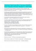
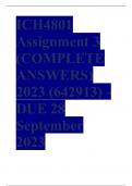
Saturation experiment (figure) – aim = to saturate the target with radioactive ligand
- Figure: [3H]DPCPX = antagonist | increasing [L*] results in more binding | separate specific vs. non-specific binding
- Determine non-specific binding in the presence of a high conc of non-radioactively labelled ligand → non-
radioactively labelled ligand will occupy target of interest → any binding from radioligand that you find, must be to
another target or to the membranes
- 𝑆𝑝𝑒𝑐𝑖𝑓𝑖𝑐 𝑏𝑖𝑛𝑑𝑖𝑛𝑔 = 𝑡𝑜𝑡𝑎𝑙 𝑏𝑖𝑛𝑑𝑖𝑛𝑔 − 𝑛𝑜𝑛 − 𝑠𝑝𝑒𝑐𝑖𝑓𝑖𝑐 𝑏𝑖𝑛𝑑𝑖𝑛𝑔
- Specific binding curve: Bmax = max number of binding sites | KD = affinity = radioligand- and receptor specific
- This type of experiment is often done once at the start of a project (because very high [L*] are used → $$$ & these
parameters do not change during the whole project)
- KD (affinity) should always be ~ the same for different cell membrane preparations (KD is specific for a LR pair)
- Bmax tells you sth about the sample you are using → e.g. membranes have different amounts of receptor
→ Endogenously expressed receptor always have a lower Bmax than genetically modified cell lines
→ Comparable KD values (under same conditions) | Different Bmax values (under same conditions)
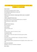
, Displacement experiment (figure) = equilibrium experiment
- Figure: displacement of agonist (CCPA) & non-radioactively labelled antagonist (DPCPX)
- Increasing conc’s of displacing ligand, will result in less radioligand binding (= what you
expect when a ligand competes for the same binding site as the radioligand)
- Figure: affinities of unlabelled compounds (agonist and antagonist)
- IC50 = inhibitory conc of ligand that results in 50% binding
- Figure: DPCPX has the highest affinity for this receptor, because more ligand is needed to reach IC50
(log -8 means a higher affinity than log -6) less antagonist is needed to displace 50% of radioligand
→ The more the curve is shifted to the left, the higher the affinity of a compound
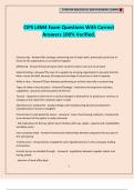
Hill-plot = linear transformation of a displacement experiment:
• Use it to get more info about the mechanism of interaction
• Hill factor (nH): says sth about type of receptor-ligand interaction
(stoichiometry) | - if it is going down | nH = (-)1.0 means there is a 1 to 1
interaction between ligand and receptor (usually the case with antagonists)
• IC50 = intercept with X-axis | depicts ligand affinity
• CCPA nH = -0.57 →
A receptor system can be depicted as a balance between active (RA) and inactive (Ri) receptors (cellular system is dynamic)
Receptor shuttles between active & inactive state in a cell → basically, you have 2 populations: active & inactive receptors
Active receptors = bound to the G-protein Inactive receptors = not bound to G-protein
In systems with genetically modified cells (high amount of receptors), there is too little G-protein → large popu of
receptors that are not bound to a G-protein & popu of receptors that has a G-protein that is endogenously available in cell
• Antagonist doesn’t discriminate between active & inactive receptor popu → binds to both equally well →
stochiometry is 1 to 1 (nH = 1.0)
• Agonist prefers to activate system → prefers to bind to active receptors
(discriminates) → stochiometry is 1 to 2 (because it sees 2 populations → nH = 0.5)
• Inverse agonist prefers to inactivate system → prefers to bind to inactive receptors
(discriminates) → stochiometry is 1 to 2 (because it sees 2 populations → nH = 0.5)
→ Antagonists & inverse agonist are often used mixed, because you need special assays to discriminate these
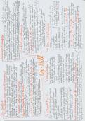
Challenge antagonistic radioligand with an antagonist displacer: antagonistic radioligand does not
discriminate → sees 2 groups → will displace RA and Ri equally well → no difference in affinity → 1 IC50
value (monophasic curve)
→ There are 2 populations, but because the have an identical IC50 value, you only see 1 IC50 value
Challenge antagonistic radioligand with an agonist displacer: agonist displacer will prefer RA over Ri
(discriminating) → with high enough conc’s of agonist displacer, it will also start displacing the antagonistic
radioligand from Ri → 1 affinity value for RA and 1 for Ri → 2 IC50 values (biphasic curve)
Challenge agonistic radioligand with either an antagonistic or agonist displacer: If you use an agonistic radioligand, you
only label the RA population → because you only label 1 population, you can only see 1 population
→ Always: 1 IC50 value (monophasic curve) → it is pharmacologically impossible to get a biphasic curve
𝐼𝐶50
Cheng-Prusoff equation: 𝐾𝑖 = 1+ [𝐿]⁄𝐾
𝐷
▪ Convert IC50 from the curve to a Ki value by correcting it for the concentration and affinity of L*
▪ Ki value (nM) becomes an independent value that can be compared between labs / assay protocols
→ Transform assay-dependent IC50 value to assay-independent Ki value
→ Antagonist has 1 Ki value | Agonist has 2 Ki values (n times more ligand needed to displace from Ri)
Kinetics of binding = association and dissociation of ligands to a receptor
→ How quickly a ligand associates to the receptor? How long does it stay at the receptor?
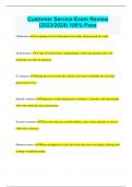
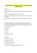
Kinetic association experiment (figure) – follow the kinetics in time (x-axis = time):
- The longer the radioligand is incubated with the receptor, the more of the radioligand will bind to the receptor
- Equilibrium plateau = where the amount of associated radioligand is equal to the amount of dissociated radioligand
→ This is not Bmax, because this is experiment is not performed under saturating concentrations
- [𝐿𝑅] = [𝐿𝑅]𝑚𝑎𝑥 ∗ (1 − 𝑒 −𝑘𝑜𝑏𝑠 ∗ 𝑡 ) = exponential equation (kobs instead of kon)
- Figure: dissociation of [3H]DPCPX by adding an excess of unlabelled ligand once the equilibrium
plateau is reached → competition for binding, but because of excess of unlabelled ligand,
[3H]DPCPX can not rebind to the receptor → dissociation of [3H]DPCPX (in time)
𝑘 ∗ 𝑡
→ [𝐿𝑅] = [𝐿𝑅]𝑡0 ∗ 𝑒 𝑜𝑓𝑓 t0 = when was experiment (with excess of unlabelled ligand) started
➔ Time-dependent & exponential
𝑘𝑜𝑏𝑠 −𝑘𝑜𝑓𝑓
- 𝑘𝑜𝑛 = [𝐿]
both experiments (association & dissociation) needed, because during association
experiment, the radioligand also dissociates → you need to correct for this dissociation & for the amount of
radioligand used in the suspension (more radioligand results in quicker association / receptor binding)
Intro
Cancer Drug Target Discovery → Computational Drug Discovery → Medicinal Chemistry → Receptor Pharmacology →
Cancer Therapeutics and Drug Safety → Image-based Computational Biology → Stem Cell Models
Aim = Discovery of novel drug targets and leads with a desired therapeutic effect and minimal adverse reactions
• Identify novel drug targets and leads through phenotypic screening for the discovery of anticancer drugs
• Establish novel safety and efficacy concepts related to the early phases of drug discovery and development
• Understand pharmacological modulation of drug targets at the molecular level
• Use computational techniques for pharmacological interaction and quantitative systems biology modelling
→ Used technologies: imaging, RNAi interference, drug screening, target discovery, cell signalling, GPCRs – kinases,
medicinal chemistry, computational biology, cheminformatics
Receptor Pharmacology
Receptor pharmacology
Drug in vivo → drug binds to target → therapeutic effect (= on-target) OR adverse effect (= off-target)
3 important questions – should be answered with yes to know whether a compound will make it to the clinic:
- Does the drug reach the site of action? - in vivo
- Does the drug bind the target? (occupancy) - in vitro assay
- Is there an on-target pharmacological effect? - in vitro assay
Drug action is all about mathematics, but you can also use Graphpad Prism
[𝐿] + [𝑅] ⇌ [𝐿𝑅] → = kon = association rate = koff = dissociation rate
Figure: association and dissociation of the ligand is a continuous process as long as the ligand is close to the target
The desired effect will only occur when the ligand & receptor are bound ([LR])
In equilibrium: 𝑘𝑜𝑛 ∗ [𝐿] ∗ [𝑅] = 𝑘𝑜𝑓𝑓 ∗ [𝐿𝑅] [L] = ligand [R] = receptor [LR] = ligand-receptor complex
→ Association determines when ligand binds to receptor | Dissociation determines how long [LR] stays together
Equilibrium dissociation constant (affinity): 𝐾𝐷 = 𝑘𝑜𝑓𝑓 ⁄𝑘𝑜𝑛 = [𝐿] ∗ [𝑅] ⁄ [𝐿𝑅] (constant = capital K)
→ More [LR] = smaller KD = higher affinity of the compound
Number of binding sites is finite → there is a max amount of binding site in the cell / in vivo
[𝑅] + [𝐿𝑅] = 𝐵𝑚𝑎𝑥
𝐵 ∗[𝐿]
[𝐿𝑅] = 𝑚𝑎𝑥 affinity & amount of ligand determine how much ligand will bind to the receptor
[𝐿]+𝐾
𝐷
→ = exponential equation: more [L] = higher [LR]
→ Plateau at some point, because [L] is in numerator & denominator
→ If [L] = KD (affinity), then you will half of your receptors occupied (Bmax / 2)
[𝐿𝑅] [𝐿]
Receptor occupancy: 𝜌𝐿 = 𝐵 = [𝐿] + 𝐾 → High [L] = high receptor occupancy
𝑚𝑎𝑥 𝐷
Measure [LR] with radioligand binding studies = label L to yield a marker (L* = radioactive, fluorescent, etc)
▪ The ideal radioligand (L*) should be: stable, tritiated, high affinity (KD ~1 nM), low non-specific binding, optimal
kinetics (temperature)
▪ Distinguish the bound ligand (L*-R) from the free ligand (L*):
- Through separation (e.g. filtration)
- Without separation (e.g. SPA)
▪ Measure [L*-R]:
- [3H], [35S]: liquid scintillation counter (use when tritiated (3H))
- [125I]: gamma counter
Saturation experiment (figure) – aim = to saturate the target with radioactive ligand
- Figure: [3H]DPCPX = antagonist | increasing [L*] results in more binding | separate specific vs. non-specific binding
- Determine non-specific binding in the presence of a high conc of non-radioactively labelled ligand → non-
radioactively labelled ligand will occupy target of interest → any binding from radioligand that you find, must be to
another target or to the membranes
- 𝑆𝑝𝑒𝑐𝑖𝑓𝑖𝑐 𝑏𝑖𝑛𝑑𝑖𝑛𝑔 = 𝑡𝑜𝑡𝑎𝑙 𝑏𝑖𝑛𝑑𝑖𝑛𝑔 − 𝑛𝑜𝑛 − 𝑠𝑝𝑒𝑐𝑖𝑓𝑖𝑐 𝑏𝑖𝑛𝑑𝑖𝑛𝑔
- Specific binding curve: Bmax = max number of binding sites | KD = affinity = radioligand- and receptor specific
- This type of experiment is often done once at the start of a project (because very high [L*] are used → $$$ & these
parameters do not change during the whole project)
- KD (affinity) should always be ~ the same for different cell membrane preparations (KD is specific for a LR pair)
- Bmax tells you sth about the sample you are using → e.g. membranes have different amounts of receptor
→ Endogenously expressed receptor always have a lower Bmax than genetically modified cell lines
→ Comparable KD values (under same conditions) | Different Bmax values (under same conditions)
, Displacement experiment (figure) = equilibrium experiment
- Figure: displacement of agonist (CCPA) & non-radioactively labelled antagonist (DPCPX)
- Increasing conc’s of displacing ligand, will result in less radioligand binding (= what you
expect when a ligand competes for the same binding site as the radioligand)
- Figure: affinities of unlabelled compounds (agonist and antagonist)
- IC50 = inhibitory conc of ligand that results in 50% binding
- Figure: DPCPX has the highest affinity for this receptor, because more ligand is needed to reach IC50
(log -8 means a higher affinity than log -6) less antagonist is needed to displace 50% of radioligand
→ The more the curve is shifted to the left, the higher the affinity of a compound
Hill-plot = linear transformation of a displacement experiment:
• Use it to get more info about the mechanism of interaction
• Hill factor (nH): says sth about type of receptor-ligand interaction
(stoichiometry) | - if it is going down | nH = (-)1.0 means there is a 1 to 1
interaction between ligand and receptor (usually the case with antagonists)
• IC50 = intercept with X-axis | depicts ligand affinity
• CCPA nH = -0.57 →
A receptor system can be depicted as a balance between active (RA) and inactive (Ri) receptors (cellular system is dynamic)
Receptor shuttles between active & inactive state in a cell → basically, you have 2 populations: active & inactive receptors
Active receptors = bound to the G-protein Inactive receptors = not bound to G-protein
In systems with genetically modified cells (high amount of receptors), there is too little G-protein → large popu of
receptors that are not bound to a G-protein & popu of receptors that has a G-protein that is endogenously available in cell
• Antagonist doesn’t discriminate between active & inactive receptor popu → binds to both equally well →
stochiometry is 1 to 1 (nH = 1.0)
• Agonist prefers to activate system → prefers to bind to active receptors
(discriminates) → stochiometry is 1 to 2 (because it sees 2 populations → nH = 0.5)
• Inverse agonist prefers to inactivate system → prefers to bind to inactive receptors
(discriminates) → stochiometry is 1 to 2 (because it sees 2 populations → nH = 0.5)
→ Antagonists & inverse agonist are often used mixed, because you need special assays to discriminate these
Challenge antagonistic radioligand with an antagonist displacer: antagonistic radioligand does not
discriminate → sees 2 groups → will displace RA and Ri equally well → no difference in affinity → 1 IC50
value (monophasic curve)
→ There are 2 populations, but because the have an identical IC50 value, you only see 1 IC50 value
Challenge antagonistic radioligand with an agonist displacer: agonist displacer will prefer RA over Ri
(discriminating) → with high enough conc’s of agonist displacer, it will also start displacing the antagonistic
radioligand from Ri → 1 affinity value for RA and 1 for Ri → 2 IC50 values (biphasic curve)
Challenge agonistic radioligand with either an antagonistic or agonist displacer: If you use an agonistic radioligand, you
only label the RA population → because you only label 1 population, you can only see 1 population
→ Always: 1 IC50 value (monophasic curve) → it is pharmacologically impossible to get a biphasic curve
𝐼𝐶50
Cheng-Prusoff equation: 𝐾𝑖 = 1+ [𝐿]⁄𝐾
𝐷
▪ Convert IC50 from the curve to a Ki value by correcting it for the concentration and affinity of L*
▪ Ki value (nM) becomes an independent value that can be compared between labs / assay protocols
→ Transform assay-dependent IC50 value to assay-independent Ki value
→ Antagonist has 1 Ki value | Agonist has 2 Ki values (n times more ligand needed to displace from Ri)
Kinetics of binding = association and dissociation of ligands to a receptor
→ How quickly a ligand associates to the receptor? How long does it stay at the receptor?
Kinetic association experiment (figure) – follow the kinetics in time (x-axis = time):
- The longer the radioligand is incubated with the receptor, the more of the radioligand will bind to the receptor
- Equilibrium plateau = where the amount of associated radioligand is equal to the amount of dissociated radioligand
→ This is not Bmax, because this is experiment is not performed under saturating concentrations
- [𝐿𝑅] = [𝐿𝑅]𝑚𝑎𝑥 ∗ (1 − 𝑒 −𝑘𝑜𝑏𝑠 ∗ 𝑡 ) = exponential equation (kobs instead of kon)
- Figure: dissociation of [3H]DPCPX by adding an excess of unlabelled ligand once the equilibrium
plateau is reached → competition for binding, but because of excess of unlabelled ligand,
[3H]DPCPX can not rebind to the receptor → dissociation of [3H]DPCPX (in time)
𝑘 ∗ 𝑡
→ [𝐿𝑅] = [𝐿𝑅]𝑡0 ∗ 𝑒 𝑜𝑓𝑓 t0 = when was experiment (with excess of unlabelled ligand) started
➔ Time-dependent & exponential
𝑘𝑜𝑏𝑠 −𝑘𝑜𝑓𝑓
- 𝑘𝑜𝑛 = [𝐿]
both experiments (association & dissociation) needed, because during association
experiment, the radioligand also dissociates → you need to correct for this dissociation & for the amount of
radioligand used in the suspension (more radioligand results in quicker association / receptor binding)