Management Research Methods 2
Lecture 1 – Conceptual models & Analysis of Variance
Clarifications
OV = Outcome Variable (Field)
o Or DV = Dependent variable
Test variable, variable to be explained
PV = Predictor Variable (Field)
o IV = Independent variable
Variable that explains
P-value
o Stands for the Probability of obtaining a result (or test-statistic value) equal to
(or ‘more extreme’ than) what was actually observed (the result you actually
got), assuming that the null hypothesis is true
o A low p value indicates that the null hypothesis is unlikely
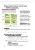
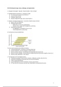
Conceptual models
o Visual representations of relationships between theoretical construct (and
variables) of interest
o In reseach: by ‘model’ we mean a simplified description of reality
o Variables can have different measurement scales:
Categorical (ordinal, nominal) – subgroups are indicated by numbers;
Quantitative (discrete, interval, ratio) – we use numerical scales, with
equal distances between values
In social sciences we sometimes treat ordinal scales as (pseudo)
interval scales, e.g. Likert scales
o ‘Communication skills’ is a moderating variable one variable moderates
the relationship between two other variables (moderation = interaction)
o ‘Lecture slides quality’ is a mediating variable one variable mediates the
relationship between two other variables
Analysis Of Variance (ANOVA)
Two measurements of variability (how much values differ in your data) are:
o Variance = the average of the squared differences from the mean (average)
o Sum of squares = the sum of the squared differences from the mean (average)
o The means are most likely to be different, but it says nothing, so you look at
the variance between groups.
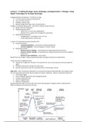
The intuition behind the ANOVA
, o MRMII students are assigned to three subgroups, each group receives a
different teaching method
o One thing could be to check if there are difference in scores on the exam
between the groups!
o What might the distribution of exam scores of the different groups look like?
o Which group scores best overall and which scores worst?
o How can we investigate with a certain level of (statistical) confidence, what
differences there might be between groups?
o This is what the ANOVA helps us to do!
It does so by comparing the variability between the groups against
the variability within the groups
In other words, does it matter in which group you are (which teaching
method you receive) with regard to your exam score?
We want variability within the groups as low as possible and variability
between the groups as high as possible
We want to see much of the variability in our outcome variable can be
explained by our predictor variable. However, we probably won’t be
able to explain all the differences (all the variability) in exam scores,
solely by creating our groups who receive different teaching methods
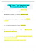
ANOVA
ANOVA statistically examines how much of the variability in our outcome variable
can be explained by our predictor variable
It breaks down different measures of variability through calculating sums of squares
Via these calculations, the ANOVA helps us test if the mean scores of the groups are
statistically different
We use (one way between-subjects) ANOVA when:
o Outcome variable (OV)= quantitative
o Predictor variable (PV)= categorical with more than 2 groups
o Variance is homogenous across groups
o Residuals are normally distributed – in this class we don’t test
o Groups are roughly equally sized – in this class they always are
o Our subjects can only be in one group (between subjects design)
NOT adhering to assumptions can produce invalid outcomes
One way ANOVA One PV
o So a Two way ANOVA can be used for?
Example:
- Research question: is there a relationship between shopping platform and customer
satisfaction?
- PV= shopping platform (categorical) – this one PV is our statistical ‘model’ in this
analysis
, o Brick-and-mortar store
o Web shop
o Reseller
- OV= customer satisfaction (quantitative)
o Score from 1-50
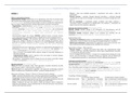
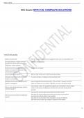
Total Sum of Squares
Imagine we have 10 observations. We have 10 observations on customer satisfaction scores
(OV)
The grand overall mean (denoted by ) is 32.3
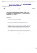
Model Sum of Squares
We now introduce our model: 1 PV (factor) with 3 levels (groups j= 1, 2 or 3)
- Independent variable= channel (1. Brick-and-mortar store, 2. Web shop, 3. Reseller)
- Model Sum of Squares = between SS=
- We have three group means, which are compared to the grand overall
mean ( is the number of observations in group j and y is the group
mean of group j. What is n1, n2 and n3?
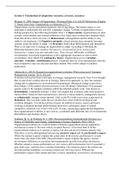
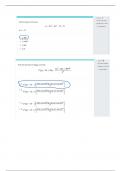
Residual Sum of Squares
Finally our model does not explain all variance in the data
- The residuals are the variances that remain in each group
, -
- If yij is the i-th observation from the j-th group (3 groups J= 3) we
have (nj 4, 3 and 3 respectively)
Sum of Squares and R2
We have now decomposed the variability in our data in a part that can be explained
by our model (between group SS) and a residual part (within group SS)
We can now calculate the proportion of the total variance in our data that is
“explained” by our model. This ratio to calculate this is called R2
’95,7% of the variability in the customer score can be explained by the type of
store’
F-test and Mean Squares
To investigate if the group means differ with an ANOVA, we do a F-test
This is a statistical test and thus checks the ratio explained variability to unexplained
variability
we want it high as possible
However, we cannot just divide the model sum of squares by the residual sum of
squares, because they are not based on the same number of observations
We therefore divide by the degrees of freedom and get something called the “mean
square”
Thus:
Look at the F-table. Column= dfmodel, row= dfresidual
As with any test statistic, the F-ratio has a null hypothesis and an alternative
hypothesis:
Lecture 1 – Conceptual models & Analysis of Variance
Clarifications
OV = Outcome Variable (Field)
o Or DV = Dependent variable
Test variable, variable to be explained
PV = Predictor Variable (Field)
o IV = Independent variable
Variable that explains
P-value
o Stands for the Probability of obtaining a result (or test-statistic value) equal to
(or ‘more extreme’ than) what was actually observed (the result you actually
got), assuming that the null hypothesis is true
o A low p value indicates that the null hypothesis is unlikely
Conceptual models
o Visual representations of relationships between theoretical construct (and
variables) of interest
o In reseach: by ‘model’ we mean a simplified description of reality
o Variables can have different measurement scales:
Categorical (ordinal, nominal) – subgroups are indicated by numbers;
Quantitative (discrete, interval, ratio) – we use numerical scales, with
equal distances between values
In social sciences we sometimes treat ordinal scales as (pseudo)
interval scales, e.g. Likert scales
o ‘Communication skills’ is a moderating variable one variable moderates
the relationship between two other variables (moderation = interaction)
o ‘Lecture slides quality’ is a mediating variable one variable mediates the
relationship between two other variables
Analysis Of Variance (ANOVA)
Two measurements of variability (how much values differ in your data) are:
o Variance = the average of the squared differences from the mean (average)
o Sum of squares = the sum of the squared differences from the mean (average)
o The means are most likely to be different, but it says nothing, so you look at
the variance between groups.
The intuition behind the ANOVA
, o MRMII students are assigned to three subgroups, each group receives a
different teaching method
o One thing could be to check if there are difference in scores on the exam
between the groups!
o What might the distribution of exam scores of the different groups look like?
o Which group scores best overall and which scores worst?
o How can we investigate with a certain level of (statistical) confidence, what
differences there might be between groups?
o This is what the ANOVA helps us to do!
It does so by comparing the variability between the groups against
the variability within the groups
In other words, does it matter in which group you are (which teaching
method you receive) with regard to your exam score?
We want variability within the groups as low as possible and variability
between the groups as high as possible
We want to see much of the variability in our outcome variable can be
explained by our predictor variable. However, we probably won’t be
able to explain all the differences (all the variability) in exam scores,
solely by creating our groups who receive different teaching methods
ANOVA
ANOVA statistically examines how much of the variability in our outcome variable
can be explained by our predictor variable
It breaks down different measures of variability through calculating sums of squares
Via these calculations, the ANOVA helps us test if the mean scores of the groups are
statistically different
We use (one way between-subjects) ANOVA when:
o Outcome variable (OV)= quantitative
o Predictor variable (PV)= categorical with more than 2 groups
o Variance is homogenous across groups
o Residuals are normally distributed – in this class we don’t test
o Groups are roughly equally sized – in this class they always are
o Our subjects can only be in one group (between subjects design)
NOT adhering to assumptions can produce invalid outcomes
One way ANOVA One PV
o So a Two way ANOVA can be used for?
Example:
- Research question: is there a relationship between shopping platform and customer
satisfaction?
- PV= shopping platform (categorical) – this one PV is our statistical ‘model’ in this
analysis
, o Brick-and-mortar store
o Web shop
o Reseller
- OV= customer satisfaction (quantitative)
o Score from 1-50
Total Sum of Squares
Imagine we have 10 observations. We have 10 observations on customer satisfaction scores
(OV)
The grand overall mean (denoted by ) is 32.3
Model Sum of Squares
We now introduce our model: 1 PV (factor) with 3 levels (groups j= 1, 2 or 3)
- Independent variable= channel (1. Brick-and-mortar store, 2. Web shop, 3. Reseller)
- Model Sum of Squares = between SS=
- We have three group means, which are compared to the grand overall
mean ( is the number of observations in group j and y is the group
mean of group j. What is n1, n2 and n3?
Residual Sum of Squares
Finally our model does not explain all variance in the data
- The residuals are the variances that remain in each group
, -
- If yij is the i-th observation from the j-th group (3 groups J= 3) we
have (nj 4, 3 and 3 respectively)
Sum of Squares and R2
We have now decomposed the variability in our data in a part that can be explained
by our model (between group SS) and a residual part (within group SS)
We can now calculate the proportion of the total variance in our data that is
“explained” by our model. This ratio to calculate this is called R2
’95,7% of the variability in the customer score can be explained by the type of
store’
F-test and Mean Squares
To investigate if the group means differ with an ANOVA, we do a F-test
This is a statistical test and thus checks the ratio explained variability to unexplained
variability
we want it high as possible
However, we cannot just divide the model sum of squares by the residual sum of
squares, because they are not based on the same number of observations
We therefore divide by the degrees of freedom and get something called the “mean
square”
Thus:
Look at the F-table. Column= dfmodel, row= dfresidual
As with any test statistic, the F-ratio has a null hypothesis and an alternative
hypothesis: