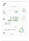
Dynamical systems
, Chapter I
&
Lecture 1|2
First order differential equations CODE)
first derivative appears
only the
f(x
· where
X(0) Xo (initial
X is a state a
variabl source : f'(x1s0 ,
tend away from
solutions
.
eq
=
condition)
Xn + 1 =
f(xn) ,
n = 0 ,7 ,2 . sink : f'(x)0 ,
solutions
tend to equilibrium
- =
aX
,
afR = x XX
= =
X(t) is an unknown real-valued function of variable to
& for each value a we
,
have a different differential equation
solution Keat
general :
X(t) =
,
KERR and K = x10) initial condition
x(t) akyat= =
aX(t)
* A no other solutions
initial value problem ([vP) : X' =
ax X 10) No =
the solution X(t) to IVP has to "solve the differential equation
2
take the valueno at t 0
=
· when K 0 the solution the constant XC = 0. > this is called the
equilibrium solution/point.
-
=
is
,
phase line
X(t) X(t)
when a changes the solutions change :
if
S
f
· a 0 :
limx( =
00 K Xo =
to
source
-
00 if K =
X 100
O if K =
x(0) =
0
~
equilibrium
* all nonzero solutions away from equili .
equilibrium
.
2 If a =
0 :
X (+) =
heat=constant X(t) X(t)
V
.
3 If aco :
lim x (H) =
0 to Sink
t+0
* all nonzero solutions tend to equili
* phase line :
XCH is a function of time ,
we can view it as a particle moving along the real line
at the
equilibrium it remains at rest (dot) ,
for any other solution it moves up or down (arrows)
the replace behavior (behavior of graph) doesn't
X stable when ato , whatever b (with a with the
qualitive change.
·
a
ax is constant same
sign as we
=
, ,
when a =
o
,
the slightest change in a leads to radical change in the behavior of solutions
Bifurcation changes of the
qualitive behavior of . A
solutions change from to this changes the equilibrium from
positive negative source
: m
to sink.
·
we have a bifurcation at a =o in the one-parameter family of equations x =
ax
, The logistic population model
For aso ,
we consider v =
ax as a simple model of population growth
.
·
x (t) measures the population of a species at time +
rate of
growth of population (directly proportional to the of population
a
·
size
logistic population growth model :
d = x =
ax/1) where a = rate of population growth when X N(very small
N
carrying capacity
=
* we consider N =
1 ~ =
ax( first order autonomous nonlinear differential equation
-S
right-side depends only on X
,
not to
solution : dx-ade
Std-Jadt
= Sa
eat For
=>
X(H)
vol
=
to we have
,
1 + k
so the solution becomes X10eat
eat
X (t) 0 X(t) 1 equilibrium
1 X10) + X10)
-
are points
#
= =
,
·
sink
f(x) =
X(1 x) -
R
source
·
solutions tent
to 1
X-0
to
00 -
tend
* > X
increasing
increasing
Constant harvesting and Bifurcations
·
Harvesting represents nation of population
Let a 1 =
then x =
X(1-x) (N 1) and we
=
consider that the population is harvested at constant rate 30
.
~ X =
X(1 x) - -
1
fn(x) bifurcation diagram :
X
1/2
X
a
U
source sink
h
em
[ > <
1/4
u
n
·
-
n