CHAPTER 7: OPTIMAL RISKY PORTFOLIOS
CHAPTER 7: OPTIMAL RISKY PORTFOLIOS
PROBLEM SETS
1. (a) and (e). Short-term rates and labor issues are factors that are common to all
firms and therefore must be considered as market risk factors. The remaining three
factors are unique to this corporation and are not a part of market risk.
2. (a) and (c). After real estate is added to the portfolio, there are four asset classes in
the portfolio: stocks, bonds, cash, and real estate. Portfolio variance now includes a
variance term for real estate returns and a covariance term for real estate returns
with returns for each of the other three asset classes. Therefore, portfolio risk is
affected by the variance (or standard deviation) of real estate returns and the
correlation between real estate returns and returns for each of the other asset
classes. (Note that the correlation between real estate returns and returns for cash is
most likely zero.)
3. (a) Answer (a) is valid because it provides the definition of the minimum variance
portfolio.
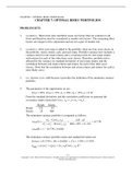
4. The parameters of the opportunity set are:
E(rS) = 20%, E(rB) = 12%, σS = 30%, σB = 15%, ρ = 0.10
From the standard deviations and the correlation coefficient we generate the
covariance matrix [note that Cov(rS , rB ) = S B ]:
Bonds Stocks
Bonds 225 45
Stocks 45 900
The minimum-variance portfolio is computed as follows:
B2 − Cov(rS ,rB ) 225 − 45
wMin(S) = = = 0.1739
S + B − 2Cov(rS ,rB ) 900 + 225 − (2 45)
2 2
wMin(B) = 1 − 0.1739 = 0.8261
The minimum variance portfolio mean and standard deviation are:
E(rMin) = (0.1739 × .20) + (0.8261 × .12) = .1339 = 13.39%
σMin = [wS2 S2 + wB2 B2 + 2wS wB Cov(rS , rB )]
7-1
Copyright © 2021 McGraw-Hill Education. All rights reserved. No reproduction or distribution without the prior written consent of
McGraw-Hill Education.
, CHAPTER 7: OPTIMAL RISKY PORTFOLIOS
= [(0.17392 900) + (0.82612 225) + (2 0.1739 0.8261 45)]1/2
= 13.92%
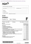
5.
Proportion Proportion Expected Standard
in Stock Fund in Bond Fund Return Deviation
0.00% 100.00% 12.00% 15.00%
17.39 82.61 13.39 13.92 minimum variance
20.00 80.00 13.60 13.94
40.00 60.00 15.20 15.70
45.16 54.84 15.61 16.54 tangency portfolio
60.00 40.00 16.80 19.53
80.00 20.00 18.40 24.48
100.00 0.00 20.00 30.00
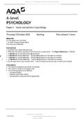
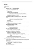
Graph shown below.
25.00
INVESTMENT OPPORTUNITY SET
20.00 CML
Tangency
Portfolio
Efficient frontier
15.00 of risky assets
10.00 Minimum
Variance
rf = 8.00 Portfolio
5.00
0.00
0.00 5.00 10.00 15.00 20.00 25.00 30.00
6. The above graph indicates that the optimal portfolio is the tangency portfolio with
expected return approximately 15.6% and standard deviation approximately 16.5%.
7-2
Copyright © 2021 McGraw-Hill Education. All rights reserved. No reproduction or distribution without the prior written consent of
McGraw-Hill Education.
CHAPTER 7: OPTIMAL RISKY PORTFOLIOS
PROBLEM SETS
1. (a) and (e). Short-term rates and labor issues are factors that are common to all
firms and therefore must be considered as market risk factors. The remaining three
factors are unique to this corporation and are not a part of market risk.
2. (a) and (c). After real estate is added to the portfolio, there are four asset classes in
the portfolio: stocks, bonds, cash, and real estate. Portfolio variance now includes a
variance term for real estate returns and a covariance term for real estate returns
with returns for each of the other three asset classes. Therefore, portfolio risk is
affected by the variance (or standard deviation) of real estate returns and the
correlation between real estate returns and returns for each of the other asset
classes. (Note that the correlation between real estate returns and returns for cash is
most likely zero.)
3. (a) Answer (a) is valid because it provides the definition of the minimum variance
portfolio.
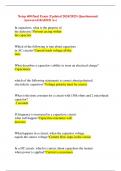
4. The parameters of the opportunity set are:
E(rS) = 20%, E(rB) = 12%, σS = 30%, σB = 15%, ρ = 0.10
From the standard deviations and the correlation coefficient we generate the
covariance matrix [note that Cov(rS , rB ) = S B ]:
Bonds Stocks
Bonds 225 45
Stocks 45 900
The minimum-variance portfolio is computed as follows:
B2 − Cov(rS ,rB ) 225 − 45
wMin(S) = = = 0.1739
S + B − 2Cov(rS ,rB ) 900 + 225 − (2 45)
2 2
wMin(B) = 1 − 0.1739 = 0.8261
The minimum variance portfolio mean and standard deviation are:
E(rMin) = (0.1739 × .20) + (0.8261 × .12) = .1339 = 13.39%
σMin = [wS2 S2 + wB2 B2 + 2wS wB Cov(rS , rB )]
7-1
Copyright © 2021 McGraw-Hill Education. All rights reserved. No reproduction or distribution without the prior written consent of
McGraw-Hill Education.
, CHAPTER 7: OPTIMAL RISKY PORTFOLIOS
= [(0.17392 900) + (0.82612 225) + (2 0.1739 0.8261 45)]1/2
= 13.92%
5.
Proportion Proportion Expected Standard
in Stock Fund in Bond Fund Return Deviation
0.00% 100.00% 12.00% 15.00%
17.39 82.61 13.39 13.92 minimum variance
20.00 80.00 13.60 13.94
40.00 60.00 15.20 15.70
45.16 54.84 15.61 16.54 tangency portfolio
60.00 40.00 16.80 19.53
80.00 20.00 18.40 24.48
100.00 0.00 20.00 30.00
Graph shown below.
25.00
INVESTMENT OPPORTUNITY SET
20.00 CML
Tangency
Portfolio
Efficient frontier
15.00 of risky assets
10.00 Minimum
Variance
rf = 8.00 Portfolio
5.00
0.00
0.00 5.00 10.00 15.00 20.00 25.00 30.00
6. The above graph indicates that the optimal portfolio is the tangency portfolio with
expected return approximately 15.6% and standard deviation approximately 16.5%.
7-2
Copyright © 2021 McGraw-Hill Education. All rights reserved. No reproduction or distribution without the prior written consent of
McGraw-Hill Education.