CHAPTER 6: RISK AVERSION AND
CAPITAL ALLOCATION TO RISKY ASSETS
CHAPTER 6: RISK AVERSION AND
CAPITAL ALLOCATION TO RISKY ASSETS
PROBLEM SETS
1. (d) While a higher or lower Sharpe ratios are not an indication of an investor's
tolerance for risk, any investor will always prefer investment portfolios with higher
Sharpe ratios. The Sharpe ratio is simply a tool to absolutely measure the return
premium earned per unit of risk.
2. (b) A higher borrowing rate is a consequence of the risk of the borrowers’ default.
In perfect markets with no additional cost of default, this increment would equal the
value of the borrower’s option to default, and the Sharpe measure, with appropriate
treatment of the default option, would be the same. However, in reality there are
costs to default so that this part of the increment lowers the Sharpe ratio. Also,
notice that answer (c) is not correct because doubling the expected return with a
fixed risk-free rate will more than double the risk premium and the Sharpe ratio.
3. Assuming no change in risk tolerance, that is, an unchanged risk-aversion
coefficient (A), higher perceived volatility increases the denominator of the
equation for the optimal investment in the risky portfolio (Equation 6.7). The
proportion invested in the risky portfolio will therefore decrease.
4. a. The expected cash flow is: (0.5 × $70,000) + (0.5 × 200,000) = $135,000.
With a risk premium of 8% over the risk-free rate of 6%, the required rate of
return is 14%. Therefore, the present value of the portfolio is:
$135,000/1.14 = $118,421
b. If the portfolio is purchased for $118,421 and provides an expected cash
inflow of $135,000, then the expected rate of return [E(r)] is as follows:
$118,421 × [1 + E(r)] = $135,000
Therefore, E(r) = 14%. The portfolio price is set to equate the expected rate of
return with the required rate of return.
c. If the risk premium over T-bills is now 12%, then the required return is:
6% + 12% = 18%
6-1
Copyright © 2021 McGraw-Hill Education. All rights reserved. No reproduction or distribution without the prior written consent of
McGraw-Hill Education.
, CHAPTER 6: RISK AVERSION AND
CAPITAL ALLOCATION TO RISKY ASSETS
The present value of the portfolio is now:
$135,000/1.18 = $114,407
d. For a given expected cash flow, portfolios that command greater risk
premiums must sell at lower prices. The extra discount from expected
value is a penalty for risk.
5. When we specify utility by U = E(r) – 0.5Aσ2, the utility level for T-bills is: 0.07
The utility level for the risky portfolio is:
U = 0.12 – 0.5 × A × (0.18)2 = 0.12 – 0.0162 × A
In order for the risky portfolio to be preferred to bills, the following must hold:
0.12 – 0.0162A > 0.07 A < 0.05/0.0162 = 3.09
A must be less than 3.09 for the risky portfolio to be preferred to bills.
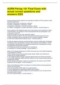
6. Points on the curve are derived by solving for E(r) in the following equation:
U = 0.05 = E(r) – 0.5Aσ2 = E(r) – 1.5σ2
The values of E(r), given the values of σ2, are therefore:
2 E(r)
0.00 0.0000 0.05000
0.05 0.0025 0.05375
0.10 0.0100 0.06500
0.15 0.0225 0.08375
0.20 0.0400 0.11000
0.25 0.0625 0.14375
The bold line in the graph on the next page (labeled Q6, for Question 6) depicts the
indifference curve.
7. Repeating the analysis in Problem 6, utility is now:
U = E(r) – 0.5Aσ2 = E(r) – 2.0σ2 = 0.05
The equal-utility combinations of expected return and standard deviation are
presented in the table below. The indifference curve is the upward sloping line in
the graph on the next page, labeled Q7 (for Question 7).
2 E(r)
6-2
Copyright © 2021 McGraw-Hill Education. All rights reserved. No reproduction or distribution without the prior written consent of
McGraw-Hill Education.
CAPITAL ALLOCATION TO RISKY ASSETS
CHAPTER 6: RISK AVERSION AND
CAPITAL ALLOCATION TO RISKY ASSETS
PROBLEM SETS
1. (d) While a higher or lower Sharpe ratios are not an indication of an investor's
tolerance for risk, any investor will always prefer investment portfolios with higher
Sharpe ratios. The Sharpe ratio is simply a tool to absolutely measure the return
premium earned per unit of risk.
2. (b) A higher borrowing rate is a consequence of the risk of the borrowers’ default.
In perfect markets with no additional cost of default, this increment would equal the
value of the borrower’s option to default, and the Sharpe measure, with appropriate
treatment of the default option, would be the same. However, in reality there are
costs to default so that this part of the increment lowers the Sharpe ratio. Also,
notice that answer (c) is not correct because doubling the expected return with a
fixed risk-free rate will more than double the risk premium and the Sharpe ratio.
3. Assuming no change in risk tolerance, that is, an unchanged risk-aversion
coefficient (A), higher perceived volatility increases the denominator of the
equation for the optimal investment in the risky portfolio (Equation 6.7). The
proportion invested in the risky portfolio will therefore decrease.
4. a. The expected cash flow is: (0.5 × $70,000) + (0.5 × 200,000) = $135,000.
With a risk premium of 8% over the risk-free rate of 6%, the required rate of
return is 14%. Therefore, the present value of the portfolio is:
$135,000/1.14 = $118,421
b. If the portfolio is purchased for $118,421 and provides an expected cash
inflow of $135,000, then the expected rate of return [E(r)] is as follows:
$118,421 × [1 + E(r)] = $135,000
Therefore, E(r) = 14%. The portfolio price is set to equate the expected rate of
return with the required rate of return.
c. If the risk premium over T-bills is now 12%, then the required return is:
6% + 12% = 18%
6-1
Copyright © 2021 McGraw-Hill Education. All rights reserved. No reproduction or distribution without the prior written consent of
McGraw-Hill Education.
, CHAPTER 6: RISK AVERSION AND
CAPITAL ALLOCATION TO RISKY ASSETS
The present value of the portfolio is now:
$135,000/1.18 = $114,407
d. For a given expected cash flow, portfolios that command greater risk
premiums must sell at lower prices. The extra discount from expected
value is a penalty for risk.
5. When we specify utility by U = E(r) – 0.5Aσ2, the utility level for T-bills is: 0.07
The utility level for the risky portfolio is:
U = 0.12 – 0.5 × A × (0.18)2 = 0.12 – 0.0162 × A
In order for the risky portfolio to be preferred to bills, the following must hold:
0.12 – 0.0162A > 0.07 A < 0.05/0.0162 = 3.09
A must be less than 3.09 for the risky portfolio to be preferred to bills.
6. Points on the curve are derived by solving for E(r) in the following equation:
U = 0.05 = E(r) – 0.5Aσ2 = E(r) – 1.5σ2
The values of E(r), given the values of σ2, are therefore:
2 E(r)
0.00 0.0000 0.05000
0.05 0.0025 0.05375
0.10 0.0100 0.06500
0.15 0.0225 0.08375
0.20 0.0400 0.11000
0.25 0.0625 0.14375
The bold line in the graph on the next page (labeled Q6, for Question 6) depicts the
indifference curve.
7. Repeating the analysis in Problem 6, utility is now:
U = E(r) – 0.5Aσ2 = E(r) – 2.0σ2 = 0.05
The equal-utility combinations of expected return and standard deviation are
presented in the table below. The indifference curve is the upward sloping line in
the graph on the next page, labeled Q7 (for Question 7).
2 E(r)
6-2
Copyright © 2021 McGraw-Hill Education. All rights reserved. No reproduction or distribution without the prior written consent of
McGraw-Hill Education.