1
TUT 2 on ANOVA and Ch 18 linked to Ch 13 MEMORANDUM
Question 1
In order to measure the intensity of sound, random samples were drawn from the
following populations (numbered in the table below) and the sound made measured in
decibels (dB):
Sample size Average Standard deviation
1 = Normal conversation 10 60 4.5
2 = A car engine 10 70 4.8
3 = An Mp3 player at maximum volume 15 105 5.5
4 = Sound of a washing machine 8 60 4.8
5 = Sound of a lawnmower 5 105 5.8
An analysis of variance (ANOVA) is conducted to determine whether differences exist
between the mean (average) sound intensity for the different sources of sound. Assume
that the necessary conditions for an analysis of variance are being met.
a) The response variable is: Sound intensity
b) The factor of this investigation is: Sources of sound
c) The number of levels of the factor is: 5
d) The number of responses is: 48
10(60)+10(70)+15(105)+8(60)+5(105) 3880
e) The overall mean intensity of sound, 𝑥𝑥̿ is: 10+10+15+8+5
= 48 =
80.8333
f) Complete the following ANOVA (to 2 decimals, if necessary) table under the assumption
that all the necessary requirements are met.
Source of Variation 𝑆𝑆𝑆𝑆 df MS F p-value
Between groups
20666.67 4 5166.67 200.34 0.0000
Within groups
1108.95 43 25.79
Total
21775.62 47
g) The alternative hypothesis will be:
A. All the population variances are the same.
B. Not all the population variances are the same.
C. At least two of the population variances differ.
D. All the population means are equal.
E. Not all population means are equal.
h) At a 5% level of significance, the decision is:
A. Do not reject 𝐻𝐻0
B. Reject 𝐻𝐻0
i) Conclusion: At a 5% level of significance, we have enough evidence to conclude that
not all population means are equal
, 2
Question 2
A well-known car magazine has decided to compare the average petrol consumption of
midsize cars between 4 independent manufacturers. It was decided to select a number of
recently produced cars randomly from each manufacturer and to subject the 16 selected cars
to identical road tests. The petrol consumption ( l100 km) is given below:
Manufacturer 1 8.8 8.9 9.3 8.9
Manufacturer 2 9.6 9.9 9.1
Manufacturer 3 9.7 8.3 8.9 9.1 8.7
Manufacturer 4 9.2 9.5 9.7 9.5
The hypothesis to be tested is whether there is a significant difference in the mean petrol
consumption of midsize cars between the 4 manufacturers based on the necessary
assumptions of normality and equal variances. Complete the following ANOVA table of
values:
Calculations (take note of intermediate rounding used):
k = number of treatments = 4
𝑛𝑛 𝑇𝑇 = 𝑛𝑛1 + 𝑛𝑛2 + 𝑛𝑛3 + 𝑛𝑛4 = 4 + 3 + 5 + 4 = 16
Overall mean:
𝑛𝑛1 𝑥𝑥1 +𝑛𝑛2 𝑥𝑥2 +𝑛𝑛3 𝑥𝑥3 +𝑛𝑛4 𝑥𝑥4 (4)(8.975)+(3)(9.5333)+(5)(8.94)+4(9.475)
𝑥𝑥̿ = = = 9.19374375 ≈ 9.1937
𝑛𝑛𝑇𝑇 16
Sum of squares due to treatments (𝑺𝑺𝑺𝑺𝑺𝑺𝑺𝑺)
2
= ∑𝑘𝑘𝑗𝑗=1 𝑛𝑛𝑗𝑗 �𝑥𝑥𝑗𝑗 − 𝑥𝑥̿ �
= 𝑛𝑛1 (𝑥𝑥1 − 𝑥𝑥̿ )2 + 𝑛𝑛2 (𝑥𝑥2 − 𝑥𝑥̿ )2 + 𝑛𝑛3 (𝑥𝑥3 − 𝑥𝑥̿ )2 + 𝑛𝑛4 (𝑥𝑥4 − 𝑥𝑥̿ )2
= 4(8.975 − 9.1937)2 + 3(9.5333 − 9.1937)2 + 5(8.94 − 9.1937)2 + 4(9.475 − 9.1937)2
= 1.1756
Mean square due to treatments (MSTR)
𝑆𝑆𝑆𝑆𝑆𝑆𝑆𝑆 1.1756
𝑀𝑀𝑀𝑀𝑀𝑀𝑀𝑀 = = = 0.3919
𝑘𝑘−1 3
Note that the MSTR is also called the: Between-treatment estimate of the population variance 𝜎𝜎 2
Sum of squares due to errors (SSE)
= ∑𝑘𝑘𝑗𝑗=1�𝑛𝑛𝑗𝑗 − 1�𝑠𝑠𝑗𝑗2
= (4 − 1)(0.0492) + (3 − 1)(0.1633) + (5 − 1)(0.268) + (4 − 1)(0.0425)
= 1.6737
Mean square due to error (MSE)
𝑆𝑆𝑆𝑆𝑆𝑆 1.6737
𝑀𝑀𝑀𝑀𝑀𝑀 = = = 0.1395
𝑛𝑛𝑇𝑇 −𝑘𝑘 12
Note that the MSE is also called the: Within-treatment estimate of the population variance 𝜎𝜎 2
SST = SSTR + SSE =1.1756+ 1.6737 = 2.8493
TUT 2 on ANOVA and Ch 18 linked to Ch 13 MEMORANDUM
Question 1
In order to measure the intensity of sound, random samples were drawn from the
following populations (numbered in the table below) and the sound made measured in
decibels (dB):
Sample size Average Standard deviation
1 = Normal conversation 10 60 4.5
2 = A car engine 10 70 4.8
3 = An Mp3 player at maximum volume 15 105 5.5
4 = Sound of a washing machine 8 60 4.8
5 = Sound of a lawnmower 5 105 5.8
An analysis of variance (ANOVA) is conducted to determine whether differences exist
between the mean (average) sound intensity for the different sources of sound. Assume
that the necessary conditions for an analysis of variance are being met.
a) The response variable is: Sound intensity
b) The factor of this investigation is: Sources of sound
c) The number of levels of the factor is: 5
d) The number of responses is: 48
10(60)+10(70)+15(105)+8(60)+5(105) 3880
e) The overall mean intensity of sound, 𝑥𝑥̿ is: 10+10+15+8+5
= 48 =
80.8333
f) Complete the following ANOVA (to 2 decimals, if necessary) table under the assumption
that all the necessary requirements are met.
Source of Variation 𝑆𝑆𝑆𝑆 df MS F p-value
Between groups
20666.67 4 5166.67 200.34 0.0000
Within groups
1108.95 43 25.79
Total
21775.62 47
g) The alternative hypothesis will be:
A. All the population variances are the same.
B. Not all the population variances are the same.
C. At least two of the population variances differ.
D. All the population means are equal.
E. Not all population means are equal.
h) At a 5% level of significance, the decision is:
A. Do not reject 𝐻𝐻0
B. Reject 𝐻𝐻0
i) Conclusion: At a 5% level of significance, we have enough evidence to conclude that
not all population means are equal
, 2
Question 2
A well-known car magazine has decided to compare the average petrol consumption of
midsize cars between 4 independent manufacturers. It was decided to select a number of
recently produced cars randomly from each manufacturer and to subject the 16 selected cars
to identical road tests. The petrol consumption ( l100 km) is given below:
Manufacturer 1 8.8 8.9 9.3 8.9
Manufacturer 2 9.6 9.9 9.1
Manufacturer 3 9.7 8.3 8.9 9.1 8.7
Manufacturer 4 9.2 9.5 9.7 9.5
The hypothesis to be tested is whether there is a significant difference in the mean petrol
consumption of midsize cars between the 4 manufacturers based on the necessary
assumptions of normality and equal variances. Complete the following ANOVA table of
values:
Calculations (take note of intermediate rounding used):
k = number of treatments = 4
𝑛𝑛 𝑇𝑇 = 𝑛𝑛1 + 𝑛𝑛2 + 𝑛𝑛3 + 𝑛𝑛4 = 4 + 3 + 5 + 4 = 16
Overall mean:
𝑛𝑛1 𝑥𝑥1 +𝑛𝑛2 𝑥𝑥2 +𝑛𝑛3 𝑥𝑥3 +𝑛𝑛4 𝑥𝑥4 (4)(8.975)+(3)(9.5333)+(5)(8.94)+4(9.475)
𝑥𝑥̿ = = = 9.19374375 ≈ 9.1937
𝑛𝑛𝑇𝑇 16
Sum of squares due to treatments (𝑺𝑺𝑺𝑺𝑺𝑺𝑺𝑺)
2
= ∑𝑘𝑘𝑗𝑗=1 𝑛𝑛𝑗𝑗 �𝑥𝑥𝑗𝑗 − 𝑥𝑥̿ �
= 𝑛𝑛1 (𝑥𝑥1 − 𝑥𝑥̿ )2 + 𝑛𝑛2 (𝑥𝑥2 − 𝑥𝑥̿ )2 + 𝑛𝑛3 (𝑥𝑥3 − 𝑥𝑥̿ )2 + 𝑛𝑛4 (𝑥𝑥4 − 𝑥𝑥̿ )2
= 4(8.975 − 9.1937)2 + 3(9.5333 − 9.1937)2 + 5(8.94 − 9.1937)2 + 4(9.475 − 9.1937)2
= 1.1756
Mean square due to treatments (MSTR)
𝑆𝑆𝑆𝑆𝑆𝑆𝑆𝑆 1.1756
𝑀𝑀𝑀𝑀𝑀𝑀𝑀𝑀 = = = 0.3919
𝑘𝑘−1 3
Note that the MSTR is also called the: Between-treatment estimate of the population variance 𝜎𝜎 2
Sum of squares due to errors (SSE)
= ∑𝑘𝑘𝑗𝑗=1�𝑛𝑛𝑗𝑗 − 1�𝑠𝑠𝑗𝑗2
= (4 − 1)(0.0492) + (3 − 1)(0.1633) + (5 − 1)(0.268) + (4 − 1)(0.0425)
= 1.6737
Mean square due to error (MSE)
𝑆𝑆𝑆𝑆𝑆𝑆 1.6737
𝑀𝑀𝑀𝑀𝑀𝑀 = = = 0.1395
𝑛𝑛𝑇𝑇 −𝑘𝑘 12
Note that the MSE is also called the: Within-treatment estimate of the population variance 𝜎𝜎 2
SST = SSTR + SSE =1.1756+ 1.6737 = 2.8493