Stochastic Modeling X 400646 period 2
Havikja van As
December 12, 2023
Contents
1 Introduction CTMC 2
2 Conditioning on the first jump 4
3 Long term behaviour 6
3.1 Stability . . . . . . . . . . . . . . . . . . . . . . . . . . . . . . . . . . . . . . . . . . . . . 8
4 Long run average cost 9
5 Queuing models 10
5.1 Kendall’s notation . . . . . . . . . . . . . . . . . . . . . . . . . . . . . . . . . . . . . . . 10
5.2 Terminology . . . . . . . . . . . . . . . . . . . . . . . . . . . . . . . . . . . . . . . . . . . 10
5.3 PASTA . . . . . . . . . . . . . . . . . . . . . . . . . . . . . . . . . . . . . . . . . . . . . 11
5.4 Little’s Law . . . . . . . . . . . . . . . . . . . . . . . . . . . . . . . . . . . . . . . . . . . 11
6 M/M/1 12
7 M/M/1/k 15
8 M/M/c/c 17
9 M/M/c 18
10 M/G/c/c 20
11 M/M/∞ and M/G/∞ 21
12 Residual waiting time 22
13 M/G/1 24
13.1 Service disciplines . . . . . . . . . . . . . . . . . . . . . . . . . . . . . . . . . . . . . . . 25
13.2 Busy period . . . . . . . . . . . . . . . . . . . . . . . . . . . . . . . . . . . . . . . . . . . 26
13.2.1 Customer busy period . . . . . . . . . . . . . . . . . . . . . . . . . . . . . . . . . 26
A Probability distributions 28
A.1 Exponential distribution . . . . . . . . . . . . . . . . . . . . . . . . . . . . . . . . . . . . 28
A.2 Poisson distribution . . . . . . . . . . . . . . . . . . . . . . . . . . . . . . . . . . . . . . 28
A.3 Erlang distribution . . . . . . . . . . . . . . . . . . . . . . . . . . . . . . . . . . . . . . . 28
B Series 29
B.1 Geometric series . . . . . . . . . . . . . . . . . . . . . . . . . . . . . . . . . . . . . . . . 29
1
,1 Introduction CTMC
A Continuous Time Markov Chain (CTMC) on a countable state space S is a process {X(t), t ≥ 0},
opposed to a sequence like a DTMC. Meaning that there are no self loops. Where X(t) is the state at
time t and t ∈ R.
Figure 1: Visual representation of a possible trajectory for a CTMC
When arriving in state i, for each state j and clock starts that represents the time until a transition to
state j is made from state i. These times are independent Exponential distributions Exp(q Pij ), where
qij is the transition rate from state i to state j and the (total) rate out of state i is νi := j qij .
A transition will be made when the first exponential clock runs out. Thus the time spent in state i is:
X
min(Exp(qij )) ∼ Exp( qij )
j
qij
and state j is the next state with probability νi .
Note that it is impossible for two exponential clocks to run out at the same time. P (Exp1 (µ) =
Exp2 (µ)) = 0
Theorem 1.1. A process as described automatically satisfies the Markov property for all times
t0 < t1 < · · · < tn < tn+1 and all states i, j, i1 , . . . , in−1 ∈ S,
P (X(tn+1 ) = j|X(t0 ) = i0 , X(t1 ) = i1 , . . . , X(tn−1 ) = in−1 ,X(tn ) = i) = P (X(tn+1 ) = j|X(tn ) = i)
Additionally, the transition rates qij are independent of t causing CTMC automatically to be Time-
homogeneous.
P (X(t) = j|X(s) = i) = P (X(t − s) = j|X(0) = i)
The checklist for formulating a CTMC:
• State X(t) := . . . at time t
• Specify the state space and the transition rates (give the transition diagram with the transition
rates when convenient).
• Motivate that all transition times are Exponential and specify how they where established
Example - Machine reliability with 2 machines
Two machines are used in production. Each of the two machines lasts for an Exp() stretch of
time before it gets broken. Once it gets broken it immediately goes into repair for an Exp(µ)
amount of time. After a repair the machine is immediately in use again before it gets broken
again. The up-times and repair-times are all independent.
Argue X(t) = number of functioning machines at time t is a CTMC.
2
, S = {0, 1, 2}
λ 2λ
0 1 2
2µ µ
• 1 → 2: When the repair time of the broken machine is over, Exp(µ)
• 1 → 0: When the working machine breaks, Exp(λ)
• 0 → 1: When the repair time of one of the broken machines is over,
min[Exp1 (µ), Exp2 (µ)] = Exp(2µ)
• 2 → 1: When one of the two working machines brakes,
min[Exp1 (λ), Exp2 (λ)] = Exp(2λ)
• 2 → 0: Not a possible transition, because it is impossible that both machines break at
exactly the same time.
Example - M/M/2/4
Customers arrive according to a P P (λ). There are 2 servers and 2 spots in the waiting
room. When both servers are bussy an arriving customer is willing to wait with probability p,
independently of other customers. When the waiting room is full the customer will not enter.
The service times of the customers are i.i.d. Exp(µ). The servers don’t idle, ie serve customers
back to back as long as there are customers in the system.
Formulate an appropriate CTMC.
X(t) := the number of customers in the system at time t.
S := {0, 1, 2, 3, 4}
Customers arrive according to a P P (λ), which means that the inter arrival time of these
customers are Exp(λ). It is given that the service times are Exp(µ).
Possible transitions:
• 4 → 3: When one of the two working servers is finished. min[Exp1 (µ), Exp2 (µ)] =
Exp(2µ)
• 3 → 2: When one of the two working servers is finished. min[Exp1 (µ), Exp2 (µ)] =
Exp(2µ)
• 2 → 1: When one of the two working servers is finished. min[Exp1 (µ), Exp2 (µ)] =
Exp(2µ)
• 1 → 0: When the working server is finished. Exp(µ)
• 0 → 1: When a customer arrives. Exp(λ)
• 1 → 2: When a customer arrives. Exp(λ)
• 2 → 3: When a customer that is willing to wait arrives. Exp(pλ)
• 3 → 4: When a customer that is willing to wait arrives. Exp(pλ)
Total rates:
• ν0 = λ
• ν1 = µ + λ
• ν2 = 2µ + λ
• ν3 = 2µ + λ
• ν4 = 2µ
µ 2µ 2µ 2µ
0 1 2 3 4
λ λ λ λ
3
Havikja van As
December 12, 2023
Contents
1 Introduction CTMC 2
2 Conditioning on the first jump 4
3 Long term behaviour 6
3.1 Stability . . . . . . . . . . . . . . . . . . . . . . . . . . . . . . . . . . . . . . . . . . . . . 8
4 Long run average cost 9
5 Queuing models 10
5.1 Kendall’s notation . . . . . . . . . . . . . . . . . . . . . . . . . . . . . . . . . . . . . . . 10
5.2 Terminology . . . . . . . . . . . . . . . . . . . . . . . . . . . . . . . . . . . . . . . . . . . 10
5.3 PASTA . . . . . . . . . . . . . . . . . . . . . . . . . . . . . . . . . . . . . . . . . . . . . 11
5.4 Little’s Law . . . . . . . . . . . . . . . . . . . . . . . . . . . . . . . . . . . . . . . . . . . 11
6 M/M/1 12
7 M/M/1/k 15
8 M/M/c/c 17
9 M/M/c 18
10 M/G/c/c 20
11 M/M/∞ and M/G/∞ 21
12 Residual waiting time 22
13 M/G/1 24
13.1 Service disciplines . . . . . . . . . . . . . . . . . . . . . . . . . . . . . . . . . . . . . . . 25
13.2 Busy period . . . . . . . . . . . . . . . . . . . . . . . . . . . . . . . . . . . . . . . . . . . 26
13.2.1 Customer busy period . . . . . . . . . . . . . . . . . . . . . . . . . . . . . . . . . 26
A Probability distributions 28
A.1 Exponential distribution . . . . . . . . . . . . . . . . . . . . . . . . . . . . . . . . . . . . 28
A.2 Poisson distribution . . . . . . . . . . . . . . . . . . . . . . . . . . . . . . . . . . . . . . 28
A.3 Erlang distribution . . . . . . . . . . . . . . . . . . . . . . . . . . . . . . . . . . . . . . . 28
B Series 29
B.1 Geometric series . . . . . . . . . . . . . . . . . . . . . . . . . . . . . . . . . . . . . . . . 29
1
,1 Introduction CTMC
A Continuous Time Markov Chain (CTMC) on a countable state space S is a process {X(t), t ≥ 0},
opposed to a sequence like a DTMC. Meaning that there are no self loops. Where X(t) is the state at
time t and t ∈ R.
Figure 1: Visual representation of a possible trajectory for a CTMC
When arriving in state i, for each state j and clock starts that represents the time until a transition to
state j is made from state i. These times are independent Exponential distributions Exp(q Pij ), where
qij is the transition rate from state i to state j and the (total) rate out of state i is νi := j qij .
A transition will be made when the first exponential clock runs out. Thus the time spent in state i is:
X
min(Exp(qij )) ∼ Exp( qij )
j
qij
and state j is the next state with probability νi .
Note that it is impossible for two exponential clocks to run out at the same time. P (Exp1 (µ) =
Exp2 (µ)) = 0
Theorem 1.1. A process as described automatically satisfies the Markov property for all times
t0 < t1 < · · · < tn < tn+1 and all states i, j, i1 , . . . , in−1 ∈ S,
P (X(tn+1 ) = j|X(t0 ) = i0 , X(t1 ) = i1 , . . . , X(tn−1 ) = in−1 ,X(tn ) = i) = P (X(tn+1 ) = j|X(tn ) = i)
Additionally, the transition rates qij are independent of t causing CTMC automatically to be Time-
homogeneous.
P (X(t) = j|X(s) = i) = P (X(t − s) = j|X(0) = i)
The checklist for formulating a CTMC:
• State X(t) := . . . at time t
• Specify the state space and the transition rates (give the transition diagram with the transition
rates when convenient).
• Motivate that all transition times are Exponential and specify how they where established
Example - Machine reliability with 2 machines
Two machines are used in production. Each of the two machines lasts for an Exp() stretch of
time before it gets broken. Once it gets broken it immediately goes into repair for an Exp(µ)
amount of time. After a repair the machine is immediately in use again before it gets broken
again. The up-times and repair-times are all independent.
Argue X(t) = number of functioning machines at time t is a CTMC.
2
, S = {0, 1, 2}
λ 2λ
0 1 2
2µ µ
• 1 → 2: When the repair time of the broken machine is over, Exp(µ)
• 1 → 0: When the working machine breaks, Exp(λ)
• 0 → 1: When the repair time of one of the broken machines is over,
min[Exp1 (µ), Exp2 (µ)] = Exp(2µ)
• 2 → 1: When one of the two working machines brakes,
min[Exp1 (λ), Exp2 (λ)] = Exp(2λ)
• 2 → 0: Not a possible transition, because it is impossible that both machines break at
exactly the same time.
Example - M/M/2/4
Customers arrive according to a P P (λ). There are 2 servers and 2 spots in the waiting
room. When both servers are bussy an arriving customer is willing to wait with probability p,
independently of other customers. When the waiting room is full the customer will not enter.
The service times of the customers are i.i.d. Exp(µ). The servers don’t idle, ie serve customers
back to back as long as there are customers in the system.
Formulate an appropriate CTMC.
X(t) := the number of customers in the system at time t.
S := {0, 1, 2, 3, 4}
Customers arrive according to a P P (λ), which means that the inter arrival time of these
customers are Exp(λ). It is given that the service times are Exp(µ).
Possible transitions:
• 4 → 3: When one of the two working servers is finished. min[Exp1 (µ), Exp2 (µ)] =
Exp(2µ)
• 3 → 2: When one of the two working servers is finished. min[Exp1 (µ), Exp2 (µ)] =
Exp(2µ)
• 2 → 1: When one of the two working servers is finished. min[Exp1 (µ), Exp2 (µ)] =
Exp(2µ)
• 1 → 0: When the working server is finished. Exp(µ)
• 0 → 1: When a customer arrives. Exp(λ)
• 1 → 2: When a customer arrives. Exp(λ)
• 2 → 3: When a customer that is willing to wait arrives. Exp(pλ)
• 3 → 4: When a customer that is willing to wait arrives. Exp(pλ)
Total rates:
• ν0 = λ
• ν1 = µ + λ
• ν2 = 2µ + λ
• ν3 = 2µ + λ
• ν4 = 2µ
µ 2µ 2µ 2µ
0 1 2 3 4
λ λ λ λ
3