Basic Macroeconomic Relationships
Chapter 13
Assumptions & Current Relevance:
Prices in modern eco = inflexible
Simplifications downward over short periods of time.
Keynes created aggregate How eco likely 2 adj 2 eco shocks over
expenditures model in Great shorter time periods.
Depression 2 explain why happened & Income Consumption &
how end.
Income Saving
Stuck –Price Model Income-Consumption (C)
Positive relationship: more cons earn
Underpinning aggregate expenditures
(after tax), more spend (but not
model reflect eco conditions in Great
necessarily all)
Depression.
Income-Savings (S)
Assume prices = fixed (price lvl cannot
Savings = not spending/part of
change).
disposable income not consumed.
Prices not declined sufficiently 2
Positive relationship: more cons earn,
boost spending & maintain output/
more income can save.
employment.
Yd = Disposable Income(DI)
Unplanned Inventory Adjs Key determinant of consumption.
Represents personal consumer income
Keynes thought unemployment of
after taxes (Yd = total income – taxes)
labour & capital caused by firms
reacting in predictable way 2
unplanned incr in inventory.
Households reduced spending –
inventory of unsold goods
Consumption Schedule
unexpectedly surged.
Amts households plan 2 spend on cons
Not slash prices & not sell fast enough
goods @ diff lvls of disposable income.
– reduce rate of production & some
Saving Schedule
close.
Amts plan 2 save (not spend on goods)
Production dec in response 2
@ diff lvls of disposable income.
unexpected inventory changes:
▪ Unexpectedly rising – cut back on
production (balance production w/
sales & prevent inventory from
exceeding capacity).
▪ Unexpectedly falling – increase
production 2 take adv of good
selling env.
, Marginal Propensity 2 Save (MPS)
Fraction of any change in disposable
income households save; equal 2
change in saving divided by change in
disposable income.
MPC + MPS = 1
▪ fraction of any income change not
consumed = saved.
MPC & MPS as slopes:
▪ MPC: numerical value of slope of
consumption schedule.
▪ MPS: numerical value of slope of
saving schedule.
45° line - line along which value
of GDP (measured horizontally) = equal
2 value of aggregate expenditures
(measured vertically).
Break-even income: lvl of disposable
income @ which households plan 2
consume all income & save none of it;
also, in income transfer programme,
level of earned income @ which
subsidy payments become zero.
Read explanation p 145
Marginal Propensity 2 Consume (MPC)
Fraction of any change in disposable
income spent on cons goods; equal 2
change in consumption divided by
change in disposable income.
Chapter 13
Assumptions & Current Relevance:
Prices in modern eco = inflexible
Simplifications downward over short periods of time.
Keynes created aggregate How eco likely 2 adj 2 eco shocks over
expenditures model in Great shorter time periods.
Depression 2 explain why happened & Income Consumption &
how end.
Income Saving
Stuck –Price Model Income-Consumption (C)
Positive relationship: more cons earn
Underpinning aggregate expenditures
(after tax), more spend (but not
model reflect eco conditions in Great
necessarily all)
Depression.
Income-Savings (S)
Assume prices = fixed (price lvl cannot
Savings = not spending/part of
change).
disposable income not consumed.
Prices not declined sufficiently 2
Positive relationship: more cons earn,
boost spending & maintain output/
more income can save.
employment.
Yd = Disposable Income(DI)
Unplanned Inventory Adjs Key determinant of consumption.
Represents personal consumer income
Keynes thought unemployment of
after taxes (Yd = total income – taxes)
labour & capital caused by firms
reacting in predictable way 2
unplanned incr in inventory.
Households reduced spending –
inventory of unsold goods
Consumption Schedule
unexpectedly surged.
Amts households plan 2 spend on cons
Not slash prices & not sell fast enough
goods @ diff lvls of disposable income.
– reduce rate of production & some
Saving Schedule
close.
Amts plan 2 save (not spend on goods)
Production dec in response 2
@ diff lvls of disposable income.
unexpected inventory changes:
▪ Unexpectedly rising – cut back on
production (balance production w/
sales & prevent inventory from
exceeding capacity).
▪ Unexpectedly falling – increase
production 2 take adv of good
selling env.
, Marginal Propensity 2 Save (MPS)
Fraction of any change in disposable
income households save; equal 2
change in saving divided by change in
disposable income.
MPC + MPS = 1
▪ fraction of any income change not
consumed = saved.
MPC & MPS as slopes:
▪ MPC: numerical value of slope of
consumption schedule.
▪ MPS: numerical value of slope of
saving schedule.
45° line - line along which value
of GDP (measured horizontally) = equal
2 value of aggregate expenditures
(measured vertically).
Break-even income: lvl of disposable
income @ which households plan 2
consume all income & save none of it;
also, in income transfer programme,
level of earned income @ which
subsidy payments become zero.
Read explanation p 145
Marginal Propensity 2 Consume (MPC)
Fraction of any change in disposable
income spent on cons goods; equal 2
change in consumption divided by
change in disposable income.