

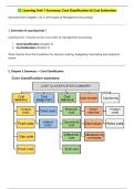
Learning Unit 1 Summary: Cost Classification & Cost Estimation
(Extracted from Chapters 2 & 3 of Principles of Management Accounting)
1. Overview of Learning Unit 1
Learning Unit 1 focuses on two core areas of management accounting:
1. Cost Classification (Chapter 2)
2. Cost Estimation (Chapter 3)
These themes form the foundation for decision-making, budgeting, forecasting and analytical
review.
2. Chapter 2 Summary — Cost Classification
,2.1 Purpose of Cost Classification
Managers classify costs to understand how decisions affect profitability. Classification helps with:
• Pricing
• Budgeting
• Cost control
• Performance evaluation
• Estimating future costs
2.2 Five Attributes of Cost Classification
(1) Cost Behaviour
Explains how costs respond to changes in activity level.
Cost Type Definition Example
Variable costs Change in proportion to level of activity Materials per student
Fixed costs Constant in total within the relevant range Lecturer fee R210 000 per year
Step costs Increase in steps as activity increases R600 per group of 5 students
Mixed costs Contain both variable & fixed elements R2 000 + R500 per student admin fees
(2) Assignment
How costs are traced to cost objects (product/service/department).
• Direct costs: Traceable (stationery, supervision).
• Indirect costs / Overheads: Not easily traceable (admin fees).
• Indirect costs require allocation.
(3) Relevance (Decision-making)
Relevant costs must be:
1. Future
2. Differential
3. Cash flows
Key concepts:
• Opportunity cost – best benefit forgone by taking the proposed course of action
• Differential cost – cost differences between alternatives
• Sunk cost – already incurred; irrelevant
,(4) Function
Used mainly for financial reporting (IAS 1 & 2).
• Inventoriable costs: Required to bring inventory to saleable condition (DM, DL, MOH)
• Non-inventoriable: Selling & admin costs
(5) Timing
• Product costs → expensed when inventory sold (absorption costing)
▪ All fixed costs is recognised as an expense in the period which they are
incurred. (variable costing)
• Period costs → expensed immediately
IAS 2 requires absorption costing for financial reporting.
3. Chapter 3 Summary — Cost Estimation
3.1 Purpose of Cost Estimation
Used to split mixed costs into fixed and variable components to forecast future costs.
3.2 Cost Drivers
A cost driver is the activity that causes a cost. Good cost drivers must be:
1. Plausible – must make sense
2. Significant – must influence the cost materially
Types of cost drivers:
• Transaction drivers (number of calls)
• Duration drivers (minutes used)
• Intensity drivers (energy used per process)
.pdf) [Principles...12 (1).pdf | PDF]
3.3 Scatter Graph Method
A visual technique to assess whether a linear relationship exists between cost and activity.
Steps:
, 1. Plot cost (Y) vs activity (X).
2. Fit a best-guess straight line.
3. Y-intercept ≈ fixed cost.
4. Slope ≈ variable cost per unit.
Used mainly to check linearity—not highly accurate.
3.4 High–Low Method
A mathematical approach using only highest and lowest activity levels.
Variable cost per unit
𝐶𝑜𝑠𝑡𝐻𝑖𝑔ℎ − 𝐶𝑜𝑠𝑡𝐿𝑜𝑤
𝑉𝐶 =
𝐴𝑐𝑡𝑖𝑣𝑖𝑡𝑦𝐻𝑖𝑔ℎ − 𝐴𝑐𝑡𝑖𝑣𝑖𝑡𝑦𝐿𝑜𝑤
Fixed cost
𝐹𝐶 = 𝑇𝑜𝑡𝑎𝑙 𝐶𝑜𝑠𝑡 − (𝑉𝐶 × 𝐴𝑐𝑡𝑖𝑣𝑖𝑡𝑦)
Useful but limited:
• Uses only two points
• Points may be unrepresentative or outside the relevant range
Linear relationship formula (also Regression equation):
y = mx + c
y – Total aggregate cost
m – Variable cost per sqm
x – cost driver level
c – fixed costs- where line intercepts the y axis
(Extracted from Chapters 2 & 3 of Principles of Management Accounting)
1. Overview of Learning Unit 1
Learning Unit 1 focuses on two core areas of management accounting:
1. Cost Classification (Chapter 2)
2. Cost Estimation (Chapter 3)
These themes form the foundation for decision-making, budgeting, forecasting and analytical
review.
2. Chapter 2 Summary — Cost Classification
,2.1 Purpose of Cost Classification
Managers classify costs to understand how decisions affect profitability. Classification helps with:
• Pricing
• Budgeting
• Cost control
• Performance evaluation
• Estimating future costs
2.2 Five Attributes of Cost Classification
(1) Cost Behaviour
Explains how costs respond to changes in activity level.
Cost Type Definition Example
Variable costs Change in proportion to level of activity Materials per student
Fixed costs Constant in total within the relevant range Lecturer fee R210 000 per year
Step costs Increase in steps as activity increases R600 per group of 5 students
Mixed costs Contain both variable & fixed elements R2 000 + R500 per student admin fees
(2) Assignment
How costs are traced to cost objects (product/service/department).
• Direct costs: Traceable (stationery, supervision).
• Indirect costs / Overheads: Not easily traceable (admin fees).
• Indirect costs require allocation.
(3) Relevance (Decision-making)
Relevant costs must be:
1. Future
2. Differential
3. Cash flows
Key concepts:
• Opportunity cost – best benefit forgone by taking the proposed course of action
• Differential cost – cost differences between alternatives
• Sunk cost – already incurred; irrelevant
,(4) Function
Used mainly for financial reporting (IAS 1 & 2).
• Inventoriable costs: Required to bring inventory to saleable condition (DM, DL, MOH)
• Non-inventoriable: Selling & admin costs
(5) Timing
• Product costs → expensed when inventory sold (absorption costing)
▪ All fixed costs is recognised as an expense in the period which they are
incurred. (variable costing)
• Period costs → expensed immediately
IAS 2 requires absorption costing for financial reporting.
3. Chapter 3 Summary — Cost Estimation
3.1 Purpose of Cost Estimation
Used to split mixed costs into fixed and variable components to forecast future costs.
3.2 Cost Drivers
A cost driver is the activity that causes a cost. Good cost drivers must be:
1. Plausible – must make sense
2. Significant – must influence the cost materially
Types of cost drivers:
• Transaction drivers (number of calls)
• Duration drivers (minutes used)
• Intensity drivers (energy used per process)
.pdf) [Principles...12 (1).pdf | PDF]
3.3 Scatter Graph Method
A visual technique to assess whether a linear relationship exists between cost and activity.
Steps:
, 1. Plot cost (Y) vs activity (X).
2. Fit a best-guess straight line.
3. Y-intercept ≈ fixed cost.
4. Slope ≈ variable cost per unit.
Used mainly to check linearity—not highly accurate.
3.4 High–Low Method
A mathematical approach using only highest and lowest activity levels.
Variable cost per unit
𝐶𝑜𝑠𝑡𝐻𝑖𝑔ℎ − 𝐶𝑜𝑠𝑡𝐿𝑜𝑤
𝑉𝐶 =
𝐴𝑐𝑡𝑖𝑣𝑖𝑡𝑦𝐻𝑖𝑔ℎ − 𝐴𝑐𝑡𝑖𝑣𝑖𝑡𝑦𝐿𝑜𝑤
Fixed cost
𝐹𝐶 = 𝑇𝑜𝑡𝑎𝑙 𝐶𝑜𝑠𝑡 − (𝑉𝐶 × 𝐴𝑐𝑡𝑖𝑣𝑖𝑡𝑦)
Useful but limited:
• Uses only two points
• Points may be unrepresentative or outside the relevant range
Linear relationship formula (also Regression equation):
y = mx + c
y – Total aggregate cost
m – Variable cost per sqm
x – cost driver level
c – fixed costs- where line intercepts the y axis


