

STA1506
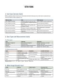
1. Fast Exam Decision Guide
When a question lands in front of you, first decide what kind of data you have. That choice usually tells you
which calculation, table or graph to use.
What you have Use Main purpose
One categorical variable Frequency table, pie chart, bar chart Show category counts or proportions
Cross-tabulation, multiple/compound
Two categorical variables Compare groups/categories
bar chart
Mean, median, mode, quartiles, SD,
One numerical variable Describe centre, spread and shape
histogram, boxplot
Show distribution or cumulative
Grouped numerical data Histogram, frequency polygon, ogive
position
Scatterplot, correlation, simple linear
Two numerical variables Study relationship/prediction
regression
Measurements over time Time-series/line plot, trend line Show trend or seasonal movement
2. Data Types and Measurement Scales
2.1 Data types
Type Meaning Examples
Qualitative / categorical Non-numerical categories Gender, blood group, car make
Quantitative Numerical data Weight, salary, age
Discrete Specific/countable numerical values Number of books, number of aircraft
Continuous Can take any value in a range Height, time, distance, salary
2.2 Measurement scales
Scale Key feature Examples Useful summaries
Nominal Categories only; no order Gender, blood group Counts, proportions, mode
Ordered categories; gaps
Ordinal Likert scale, grades Counts, proportions, mode
not measurable
Ordered; meaningful Counts, proportions, mode,
Interval °C, time of day
differences; no true zero median
Interval properties plus true Mean, median, variance,
Ratio Height, age, weight, salary
zero standard deviation
Memory trick: N → O → I → R = Name → Order → Interval → Real zero.
3. Which Graph Should I Use?
Graph Best for What it shows Key exam note
Best when categories form
Pie chart One categorical variable Part-to-whole / percentages
one total
Bar chart Categorical data Compare frequencies Bars are separate
Multiple/compound bar Compare groups across Usually built from a cross-
Two categorical variables
chart categories tabulation
Small discrete numerical Shape, clusters, common Individual values remain
Dot plot
dataset values visible
, Continuous/grouped Bars touch; class intervals
Histogram Distribution shape
numerical data on x-axis
Frequency polygon Grouped numerical data Shape of distribution Use class midpoints
Cumulative
Ogive Cumulative position Use upper class limits
frequency/percentage
Median, quartiles, spread, Useful for skewness and
Boxplot Numerical data
outliers unusual values
Direction/strength of
Scatterplot Two quantitative variables X horizontal, Y vertical
relationship
Time-series plot Values measured over time Trend and seasonality Time goes on horizontal axis
3.1 Bar chart vs histogram
• Bar chart: used for categories; bars are normally separated.
• Histogram: used for numerical class intervals; bars should touch.
• In Excel, the guide specifically instructs reducing histogram Gap Width to 0%.
4. Core Formula Sheet
Measure Formula/idea Excel Interpretation
Average value; affected by
Mean ̄ x = Σx / n =AVERAGE(range)
extreme values/outliers.
50% of observations are at
Median Middle ordered value =MEDIAN(range) or below it; less affected by
outliers.
A dataset can have none,
Mode Most frequent value =MODE.SNGL(range)
one, or multiple modes.
Also
Minimum Smallest value =MIN(range)
=QUARTILE.INC(range,0).
Also
Maximum Largest value =MAX(range)
=QUARTILE.INC(range,4).
About 25% of values are at
Q1 25th percentile =QUARTILE.INC(range,1)
or below Q1.
Divides the ordered data in
Q2 50th percentile = median =QUARTILE.INC(range,2)
half.
About 75% of values are at
Q3 75th percentile =QUARTILE.INC(range,3)
or below Q3.
Write k as decimal, e.g. 0.70
Percentile Pk =PERCENTILE.INC(range,k)
for 70th percentile.
Range Maximum − Minimum =MAX(range)-MIN(range) Overall spread.
Spread of middle 50%; not
IQR Q3 − Q1 Q3 cell − Q1 cell strongly affected by
outliers.
Variation around the mean;
Sample variance s² =VAR.S(range)
affected by outliers.
Typical spread in the
Sample standard deviation s = √s² =STDEV.S(range)
original units.
Relative variability; often
Coefficient of variation CV = s / ̄ x SD cell / Mean cell
multiply by 100 for %.
Strength and direction of
Correlation −1 ≤ r ≤ 1 =CORREL(Xrange,Yrange)
linear association.
Regression equation ŷ = a + bx INTERCEPT + SLOPE a = intercept; b = slope.
Intercept a =INTERCEPT(Yrange,Xrange) Predicted Y when X = 0.
Change in predicted Y for a
Slope b =SLOPE(Yrange,Xrange)
1-unit increase in X.
1. Fast Exam Decision Guide
When a question lands in front of you, first decide what kind of data you have. That choice usually tells you
which calculation, table or graph to use.
What you have Use Main purpose
One categorical variable Frequency table, pie chart, bar chart Show category counts or proportions
Cross-tabulation, multiple/compound
Two categorical variables Compare groups/categories
bar chart
Mean, median, mode, quartiles, SD,
One numerical variable Describe centre, spread and shape
histogram, boxplot
Show distribution or cumulative
Grouped numerical data Histogram, frequency polygon, ogive
position
Scatterplot, correlation, simple linear
Two numerical variables Study relationship/prediction
regression
Measurements over time Time-series/line plot, trend line Show trend or seasonal movement
2. Data Types and Measurement Scales
2.1 Data types
Type Meaning Examples
Qualitative / categorical Non-numerical categories Gender, blood group, car make
Quantitative Numerical data Weight, salary, age
Discrete Specific/countable numerical values Number of books, number of aircraft
Continuous Can take any value in a range Height, time, distance, salary
2.2 Measurement scales
Scale Key feature Examples Useful summaries
Nominal Categories only; no order Gender, blood group Counts, proportions, mode
Ordered categories; gaps
Ordinal Likert scale, grades Counts, proportions, mode
not measurable
Ordered; meaningful Counts, proportions, mode,
Interval °C, time of day
differences; no true zero median
Interval properties plus true Mean, median, variance,
Ratio Height, age, weight, salary
zero standard deviation
Memory trick: N → O → I → R = Name → Order → Interval → Real zero.
3. Which Graph Should I Use?
Graph Best for What it shows Key exam note
Best when categories form
Pie chart One categorical variable Part-to-whole / percentages
one total
Bar chart Categorical data Compare frequencies Bars are separate
Multiple/compound bar Compare groups across Usually built from a cross-
Two categorical variables
chart categories tabulation
Small discrete numerical Shape, clusters, common Individual values remain
Dot plot
dataset values visible
, Continuous/grouped Bars touch; class intervals
Histogram Distribution shape
numerical data on x-axis
Frequency polygon Grouped numerical data Shape of distribution Use class midpoints
Cumulative
Ogive Cumulative position Use upper class limits
frequency/percentage
Median, quartiles, spread, Useful for skewness and
Boxplot Numerical data
outliers unusual values
Direction/strength of
Scatterplot Two quantitative variables X horizontal, Y vertical
relationship
Time-series plot Values measured over time Trend and seasonality Time goes on horizontal axis
3.1 Bar chart vs histogram
• Bar chart: used for categories; bars are normally separated.
• Histogram: used for numerical class intervals; bars should touch.
• In Excel, the guide specifically instructs reducing histogram Gap Width to 0%.
4. Core Formula Sheet
Measure Formula/idea Excel Interpretation
Average value; affected by
Mean ̄ x = Σx / n =AVERAGE(range)
extreme values/outliers.
50% of observations are at
Median Middle ordered value =MEDIAN(range) or below it; less affected by
outliers.
A dataset can have none,
Mode Most frequent value =MODE.SNGL(range)
one, or multiple modes.
Also
Minimum Smallest value =MIN(range)
=QUARTILE.INC(range,0).
Also
Maximum Largest value =MAX(range)
=QUARTILE.INC(range,4).
About 25% of values are at
Q1 25th percentile =QUARTILE.INC(range,1)
or below Q1.
Divides the ordered data in
Q2 50th percentile = median =QUARTILE.INC(range,2)
half.
About 75% of values are at
Q3 75th percentile =QUARTILE.INC(range,3)
or below Q3.
Write k as decimal, e.g. 0.70
Percentile Pk =PERCENTILE.INC(range,k)
for 70th percentile.
Range Maximum − Minimum =MAX(range)-MIN(range) Overall spread.
Spread of middle 50%; not
IQR Q3 − Q1 Q3 cell − Q1 cell strongly affected by
outliers.
Variation around the mean;
Sample variance s² =VAR.S(range)
affected by outliers.
Typical spread in the
Sample standard deviation s = √s² =STDEV.S(range)
original units.
Relative variability; often
Coefficient of variation CV = s / ̄ x SD cell / Mean cell
multiply by 100 for %.
Strength and direction of
Correlation −1 ≤ r ≤ 1 =CORREL(Xrange,Yrange)
linear association.
Regression equation ŷ = a + bx INTERCEPT + SLOPE a = intercept; b = slope.
Intercept a =INTERCEPT(Yrange,Xrange) Predicted Y when X = 0.
Change in predicted Y for a
Slope b =SLOPE(Yrange,Xrange)
1-unit increase in X.


