TOPIC 3: Multilevel Analysis
______________________________________________________
In multi-level analysis, data is structured at multiple levels. The analysis accounts for this nested
structure. Examples of hierarchical data:
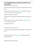
1. Implicit hierarchy of data:
Example: Students at their schools
Lower level (1): Individual students and the characteristics specific to each student
(age, gender, IQ). Things that are different per subject
Higher level (2): Groups of students (classes, schools). The characteristics are
constant for all students within the same group but can vary across different groups
(classes, school)
Researchers are interested in how level 1 variables are associated with educational
outcomes. They want to consider how group-level (2) variables influence these outcomes.
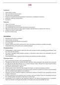
2. Explicit stage sampling data:
In longitudinal data, subjects and their multiple measures are present, and the data has
some hierarchy.
Lower level (1): Individual occasions/observations. These are the repeated measures
for each individual over time. Focus within the individual.
= Things measured that can change over time, like mood, test score, and health.
Higher level (2): Individuals: Each individual is the unit of analysis. Characteristics
that are constant over time are age, gender, and personality.
= Variables that remain stable or change slowly over time. These are the same for all
occasions over time measured for an individual.
The difference between levels:
Lowest level (Level 1): Variables where changes occur per individual/ measurement. It can change in
every condition.
Focus on variation within individuals.
Can vary widely
Higher level (Level 2): Variables that are more stable dependent on the group where they are in.
Variables may vary between different groups.
In this level, you have clusters. These are groups to which individuals belong.
You don’t necessarily need the same number of people in each group.
There is less variability within the same group. There is more variability between groups.
More complex hierarchical structures:
Three-level or higher-level data: E.g., pupils > classes > schools
Cross-classified data: Combined.
, For example, pupils in a certain neighbourhood go to a particular school. The schools and the
neighbourhood are not nested, but there are still two levels (neighbourhood> students and
students > schools).
The hierarchy depends on the definition of the variables. It is important to define the hierarchy first.
Problem with hierarchical data: Observations within a cluster are correlated
Residuals should follow a random pattern (for linear regression). With correlated
data, this is not the case
Linear regression uses total variance as error variance
Would lead to incorrect SEs and p-values for regression coefficients when not taking
into account intra-class correlation
Underestimated SEs and inflated type-I error rates
When is the correlation larger?
Small differences within clusters
Large differences between clusters
Solution: Allowing for the distinction between within-cluster and between-cluster variances to
provide correct SEs and p-values:
Within clusters: Variance at lower level
Between clusters: Variance at a higher level
Total variance: Combination of these two
How it helps (preview):
1. Including random effects: To account for variability between clusters:
Random intercepts allow each cluster to have its baseline level. Clusters may differ
systematically from one another.
2. Including fixed effects: To estimate the average relation between predictors and outcomes
across all clusters.
3. Partitioning variance: Into within- and between-cluster components. This helps to
understand the total variance.
Benefits Multi-Level Modeling:
- Using correct SEs and P-values But no big effect on estimating regression coefficients
- Ask richer questions:
Within-person changes: Pattern change & time-varying covariates
Inter-individual differences: Change patterns between individuals and associated
factors.
Starting point differences & change rate differences
- Practical reason: Handling various types of data & missing data
Leads to more dependency among observations.
, RM-ANOVA is an often-used method to analyze repeated measures in longitudinal data.
Limitations of M(ANOVA):
RM-ANOVA assumes sphericity or compound symmetry. This means the variances of the
differences between all pairs are equal. This assumption is often unrealistic in real-world
data.
o RM-ANOVA equals a random intercept model (not random slopes). However, it
cannot model individual differences in change rates over time.
RM-ANOVA requires a balanced design where all subjects are measured at the same set of
time points. This is often not the case in longitudinal studies, where some may miss certain
time points.
o RM-ANOVA cannot capture the relation between age and response in a longitudinal
design.
RM-ANOVA cannot handle missing data. Subjects that are removed reduce sample size and
introduce bias.
RM-ANOVA cannot handle non-normally distributed data. It struggles with data like
dichotomous variables, scales, and sum scores.
RM-ANOVA cannot handle time-varying predictors
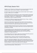
Steps for analysing longitudinal data (multi-level):
Step 1: Data format & loading the data
Two ways of formatting longitudinal data:
Wide format (person-level) = Each data line represents a single person. All observations and scores
are arranged in columns and used in simple analyses and summary statistics.
Problematic when persons are measured at different time points
Problematic when the number of time points differs between persons (missing data)
How to represent time-varying covariates?
Software often cannot read this format
Long format (person-period): Each data line represents a combination of persons and an
observation (time point). This has separate rows for each observation. A person has as many data
lines as observations available for that person.
This is the one the programs can
read.
______________________________________________________
In multi-level analysis, data is structured at multiple levels. The analysis accounts for this nested
structure. Examples of hierarchical data:
1. Implicit hierarchy of data:
Example: Students at their schools
Lower level (1): Individual students and the characteristics specific to each student
(age, gender, IQ). Things that are different per subject
Higher level (2): Groups of students (classes, schools). The characteristics are
constant for all students within the same group but can vary across different groups
(classes, school)
Researchers are interested in how level 1 variables are associated with educational
outcomes. They want to consider how group-level (2) variables influence these outcomes.
2. Explicit stage sampling data:
In longitudinal data, subjects and their multiple measures are present, and the data has
some hierarchy.
Lower level (1): Individual occasions/observations. These are the repeated measures
for each individual over time. Focus within the individual.
= Things measured that can change over time, like mood, test score, and health.
Higher level (2): Individuals: Each individual is the unit of analysis. Characteristics
that are constant over time are age, gender, and personality.
= Variables that remain stable or change slowly over time. These are the same for all
occasions over time measured for an individual.
The difference between levels:
Lowest level (Level 1): Variables where changes occur per individual/ measurement. It can change in
every condition.
Focus on variation within individuals.
Can vary widely
Higher level (Level 2): Variables that are more stable dependent on the group where they are in.
Variables may vary between different groups.
In this level, you have clusters. These are groups to which individuals belong.
You don’t necessarily need the same number of people in each group.
There is less variability within the same group. There is more variability between groups.
More complex hierarchical structures:
Three-level or higher-level data: E.g., pupils > classes > schools
Cross-classified data: Combined.
, For example, pupils in a certain neighbourhood go to a particular school. The schools and the
neighbourhood are not nested, but there are still two levels (neighbourhood> students and
students > schools).
The hierarchy depends on the definition of the variables. It is important to define the hierarchy first.
Problem with hierarchical data: Observations within a cluster are correlated
Residuals should follow a random pattern (for linear regression). With correlated
data, this is not the case
Linear regression uses total variance as error variance
Would lead to incorrect SEs and p-values for regression coefficients when not taking
into account intra-class correlation
Underestimated SEs and inflated type-I error rates
When is the correlation larger?
Small differences within clusters
Large differences between clusters
Solution: Allowing for the distinction between within-cluster and between-cluster variances to
provide correct SEs and p-values:
Within clusters: Variance at lower level
Between clusters: Variance at a higher level
Total variance: Combination of these two
How it helps (preview):
1. Including random effects: To account for variability between clusters:
Random intercepts allow each cluster to have its baseline level. Clusters may differ
systematically from one another.
2. Including fixed effects: To estimate the average relation between predictors and outcomes
across all clusters.
3. Partitioning variance: Into within- and between-cluster components. This helps to
understand the total variance.
Benefits Multi-Level Modeling:
- Using correct SEs and P-values But no big effect on estimating regression coefficients
- Ask richer questions:
Within-person changes: Pattern change & time-varying covariates
Inter-individual differences: Change patterns between individuals and associated
factors.
Starting point differences & change rate differences
- Practical reason: Handling various types of data & missing data
Leads to more dependency among observations.
, RM-ANOVA is an often-used method to analyze repeated measures in longitudinal data.
Limitations of M(ANOVA):
RM-ANOVA assumes sphericity or compound symmetry. This means the variances of the
differences between all pairs are equal. This assumption is often unrealistic in real-world
data.
o RM-ANOVA equals a random intercept model (not random slopes). However, it
cannot model individual differences in change rates over time.
RM-ANOVA requires a balanced design where all subjects are measured at the same set of
time points. This is often not the case in longitudinal studies, where some may miss certain
time points.
o RM-ANOVA cannot capture the relation between age and response in a longitudinal
design.
RM-ANOVA cannot handle missing data. Subjects that are removed reduce sample size and
introduce bias.
RM-ANOVA cannot handle non-normally distributed data. It struggles with data like
dichotomous variables, scales, and sum scores.
RM-ANOVA cannot handle time-varying predictors
Steps for analysing longitudinal data (multi-level):
Step 1: Data format & loading the data
Two ways of formatting longitudinal data:
Wide format (person-level) = Each data line represents a single person. All observations and scores
are arranged in columns and used in simple analyses and summary statistics.
Problematic when persons are measured at different time points
Problematic when the number of time points differs between persons (missing data)
How to represent time-varying covariates?
Software often cannot read this format
Long format (person-period): Each data line represents a combination of persons and an
observation (time point). This has separate rows for each observation. A person has as many data
lines as observations available for that person.
This is the one the programs can
read.