Chapter 1
Friday, January 10, 2020 5:21 PM
• Data = signal + noise
• Lurking variable (confounding) ; variable that has an important effect on the relationship among the variables in a study but is not included among the
variables studied
• Operational definition; clear, concise detailed definition of a measure
- Fundamental when collecting data
• 2 broad categories of statistics
➢ Descriptive : use of numerical and graphical methods to summarize the information revealed in the data, and present it in a convenient form
➢ Inferential: involves making estimates, decisions, predictions and other generalizations about a population based on the study of a sample (subs
of that population (set of data)
• Types of data
➢ Categorical data (qualitative)
▪ Nominal data; gives a name or number to individuals or mutually exclusive (no overlap) categories
- Categorical but appears to be numerical
➢ Numerical data (quantitative)
▪ Ordinal data; mutually exclusive categories with a fixed order (ranked)
- Letter grades
▪ Interval ; mutually exclusive, with a fixed order and equal spacing between categories
- Celsius scale, Fahrenheit scale
▪ Ratio data; mutually exclusive, with a fixed order, equal spacing between categories, and with an absolute zero point
- Height, weight, area, pressure
➢ Dichotomous (binary) : data which can take on only 2 levels or settings
▪ Sex, handedness
▪ Data can be dichotomized
STAT263 Page 1
,Chapter 2- Summarizing data: listing and grouping
Friday, January 10, 2020 6:21 PM
⚫ Statistics;
○ Location
○ Variability (spread outed-ness
○ Shape (bell-shaped, skewed)
○ If outliers (unusual values) are present
⚫ Dot plot or dot diagram = good display for relatively few data values (<50)
Data set A
⚫ Stem and leaf diagram
○ Statistical technique for displaying a set of data
○ Each numerical value is divided into 2 parts; the leading digit(s) becomes the stem and the trailing digit(s) the leaf
• advantage of stem and leaf display over
a frequency distribution = don't lose the
exact value of each observation
Minitab display:
• Shows the cumulative
frequency from each
end of the distribution Ex, 13 values in the 40s or below
and the stem which
contains the median MEDIAN is in this bin
value
Ex:
Lurking variable; how long the gynecologist has been practicing
STAT263 Page 2
, Lurking variable; how long the gynecologist has been practicing
⚫ Construction of a frequency distribution
○ Choose the classes (usually from 5-15)
▪ Largest value - smallest value = range
○ Range divided by approximate number of classes = approximate class interval or "bin width"
○ Examine the data to get practical class interval and boundaries
○ Sort or tally the data
○ Count the number of items in each class
*Rule often suggested for data sets with <200 values is to use the square root of the number of data values to find the approximate number of bins
EXAMPLE
245-76 = 169
n=80 , sqrt 80 ~ 9 = 9 approximate # of bins
169/0=18.777
*Use bin width of 20
Start the first bin at 70 (uses 9 bins)
• Cumulative frequency distribution column shows how
many values fell in the corresponding bin or below
^size of sample
STAT263 Page 3
, Would rather know the relative frequency over the frequency as it
provides more information about the data
*Shape of the frequency distribution and relative frequency distribution is the same
⚫ Histogram
*Taking midpoint
STAT263 Page 4
Friday, January 10, 2020 5:21 PM
• Data = signal + noise
• Lurking variable (confounding) ; variable that has an important effect on the relationship among the variables in a study but is not included among the
variables studied
• Operational definition; clear, concise detailed definition of a measure
- Fundamental when collecting data
• 2 broad categories of statistics
➢ Descriptive : use of numerical and graphical methods to summarize the information revealed in the data, and present it in a convenient form
➢ Inferential: involves making estimates, decisions, predictions and other generalizations about a population based on the study of a sample (subs
of that population (set of data)
• Types of data
➢ Categorical data (qualitative)
▪ Nominal data; gives a name or number to individuals or mutually exclusive (no overlap) categories
- Categorical but appears to be numerical
➢ Numerical data (quantitative)
▪ Ordinal data; mutually exclusive categories with a fixed order (ranked)
- Letter grades
▪ Interval ; mutually exclusive, with a fixed order and equal spacing between categories
- Celsius scale, Fahrenheit scale
▪ Ratio data; mutually exclusive, with a fixed order, equal spacing between categories, and with an absolute zero point
- Height, weight, area, pressure
➢ Dichotomous (binary) : data which can take on only 2 levels or settings
▪ Sex, handedness
▪ Data can be dichotomized
STAT263 Page 1
,Chapter 2- Summarizing data: listing and grouping
Friday, January 10, 2020 6:21 PM
⚫ Statistics;
○ Location
○ Variability (spread outed-ness
○ Shape (bell-shaped, skewed)
○ If outliers (unusual values) are present
⚫ Dot plot or dot diagram = good display for relatively few data values (<50)
Data set A
⚫ Stem and leaf diagram
○ Statistical technique for displaying a set of data
○ Each numerical value is divided into 2 parts; the leading digit(s) becomes the stem and the trailing digit(s) the leaf
• advantage of stem and leaf display over
a frequency distribution = don't lose the
exact value of each observation
Minitab display:
• Shows the cumulative
frequency from each
end of the distribution Ex, 13 values in the 40s or below
and the stem which
contains the median MEDIAN is in this bin
value
Ex:
Lurking variable; how long the gynecologist has been practicing
STAT263 Page 2
, Lurking variable; how long the gynecologist has been practicing
⚫ Construction of a frequency distribution
○ Choose the classes (usually from 5-15)
▪ Largest value - smallest value = range
○ Range divided by approximate number of classes = approximate class interval or "bin width"
○ Examine the data to get practical class interval and boundaries
○ Sort or tally the data
○ Count the number of items in each class
*Rule often suggested for data sets with <200 values is to use the square root of the number of data values to find the approximate number of bins
EXAMPLE
245-76 = 169
n=80 , sqrt 80 ~ 9 = 9 approximate # of bins
169/0=18.777
*Use bin width of 20
Start the first bin at 70 (uses 9 bins)
• Cumulative frequency distribution column shows how
many values fell in the corresponding bin or below
^size of sample
STAT263 Page 3
, Would rather know the relative frequency over the frequency as it
provides more information about the data
*Shape of the frequency distribution and relative frequency distribution is the same
⚫ Histogram
*Taking midpoint
STAT263 Page 4