Tilburg University
Statistics for EOR
Summary Course Material
Author: Supervisor:
Rick Smeets van Soest, A
April 2, 2024
,Table of Contents
1 Confidence Intervals 2
1.1 Pivotal Quantities . . . . . . . . . . . . . . . . . . . . . . . . . 2
1.1.1 Example No. 1 (11.1): σ 2 known, normal distribution . 3
1.1.2 Example No. 2 (11.1): σ 2 unknown, normal distribution 3
1.1.3 Example No. 3 (11.3): θ unknown, exponential distri-
bution . . . . . . . . . . . . . . . . . . . . . . . . . . . 4
1.1.4 Example No 4: finding pivotal quantities . . . . . . . . 5
1.2 Approximate Confidence Intervals . . . . . . . . . . . . . . . . 5
1.2.1 Example No. 5: asymptotic confidence interval . . . . 6
1.2.2 Example No. 6 (11.11) . . . . . . . . . . . . . . . . . . 7
1.3 Confidence intervals in two-sample problems . . . . . . . . . . 7
1.3.1 Example No. 7 (11.20) . . . . . . . . . . . . . . . . . . 9
1.4 Paired observations . . . . . . . . . . . . . . . . . . . . . . . . 9
1.5 Two Bernoulli-distributed random samples . . . . . . . . . . . 10
1.6 Non-Parametric Confidence Intervals . . . . . . . . . . . . . . 10
2 Hypothesis Testing 11
2.1 Testing for normal distributions . . . . . . . . . . . . . . . . . 12
2.2 Testing for binomial distributions . . . . . . . . . . . . . . . . 13
2.3 Uniformly most powerful tests . . . . . . . . . . . . . . . . . . 13
2.4 UMPU tests . . . . . . . . . . . . . . . . . . . . . . . . . . . . 15
3 Contingency tables 15
3.1 Test for homogeneity . . . . . . . . . . . . . . . . . . . . . . . 15
3.2 Test for independence . . . . . . . . . . . . . . . . . . . . . . . 16
4 Interpreting SPSS tables 16
5 Non-parametric tests 17
5.1 Wilcoxon signed-rank test . . . . . . . . . . . . . . . . . . . . 17
5.2 Wilcoxon/Mann-Whitney test . . . . . . . . . . . . . . . . . . 17
1
, 1 Confidence Intervals
A confidence interval (short CI) is used to estimate a parameter in such a
manner that there is a high probability that the true value of the parameter
lies in the interval. For a so called two-sided confidence interval, we have
Pθ [l(X) < τ (θ) < r(X)] = γ and define α = 1−γ. The value for γ is normally
fixed and is often a high number like 0.9, 0.95 or 0.99. Sometimes we need
one-sided confidence intervals. If Pθ [τ (θ) > l(X)] = γ then (l(x), ∞) is
called a left-sided 100γ% CI for τ (θ). In the same way, (−∞, r(x)) is called
a right-sided CI for τ (θ) if Pθ [τ (θ) < r(X)] = γ. The lenght of a CI is given
by r(X) − l(X).
For instance, a 95% confidence interval means that if we apply the procedure
many times, in about 95% of the cases the true value will lie in the confidence
interval. So, on average, we catch the true value in 95% of the cases.
There are a few important values which are being used consistently through-
out this chapter:
z0.90 = Φ−1 (0.90) = 1.282
z0.95 = Φ−1 (0.95) = 1.645
z0.975 = Φ−1 (0.975) = 1.960
z0.99 = Φ−1 (0.99) = 2.326
Moreover, note that Φ−1 ( α2 ) = −Φ−1 (1 − α2 ).
1.1 Pivotal Quantities
Q = q(X, θ) is a pivotal quantity if the probability distribution of Q does
not depend on θ. Note that Q is a function of both X and θ, so when you
write down Q, you will see a θ. The pivotal quantity Q could for instance
have a normal, chi-squared or a t-distribution. There are a few statements
with respect to a pivotal quantity.
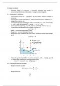
1. If θ is a one-dimensional location parameter and θ̂ is the MLE, then θ̂ − θ
is a pivotal quantity.
θ̂
2. If θ > 0 is a one-dimensional scale parameter and θ̂ is the MLE, then θ
is
a pivotal quantity.
2
Statistics for EOR
Summary Course Material
Author: Supervisor:
Rick Smeets van Soest, A
April 2, 2024
,Table of Contents
1 Confidence Intervals 2
1.1 Pivotal Quantities . . . . . . . . . . . . . . . . . . . . . . . . . 2
1.1.1 Example No. 1 (11.1): σ 2 known, normal distribution . 3
1.1.2 Example No. 2 (11.1): σ 2 unknown, normal distribution 3
1.1.3 Example No. 3 (11.3): θ unknown, exponential distri-
bution . . . . . . . . . . . . . . . . . . . . . . . . . . . 4
1.1.4 Example No 4: finding pivotal quantities . . . . . . . . 5
1.2 Approximate Confidence Intervals . . . . . . . . . . . . . . . . 5
1.2.1 Example No. 5: asymptotic confidence interval . . . . 6
1.2.2 Example No. 6 (11.11) . . . . . . . . . . . . . . . . . . 7
1.3 Confidence intervals in two-sample problems . . . . . . . . . . 7
1.3.1 Example No. 7 (11.20) . . . . . . . . . . . . . . . . . . 9
1.4 Paired observations . . . . . . . . . . . . . . . . . . . . . . . . 9
1.5 Two Bernoulli-distributed random samples . . . . . . . . . . . 10
1.6 Non-Parametric Confidence Intervals . . . . . . . . . . . . . . 10
2 Hypothesis Testing 11
2.1 Testing for normal distributions . . . . . . . . . . . . . . . . . 12
2.2 Testing for binomial distributions . . . . . . . . . . . . . . . . 13
2.3 Uniformly most powerful tests . . . . . . . . . . . . . . . . . . 13
2.4 UMPU tests . . . . . . . . . . . . . . . . . . . . . . . . . . . . 15
3 Contingency tables 15
3.1 Test for homogeneity . . . . . . . . . . . . . . . . . . . . . . . 15
3.2 Test for independence . . . . . . . . . . . . . . . . . . . . . . . 16
4 Interpreting SPSS tables 16
5 Non-parametric tests 17
5.1 Wilcoxon signed-rank test . . . . . . . . . . . . . . . . . . . . 17
5.2 Wilcoxon/Mann-Whitney test . . . . . . . . . . . . . . . . . . 17
1
, 1 Confidence Intervals
A confidence interval (short CI) is used to estimate a parameter in such a
manner that there is a high probability that the true value of the parameter
lies in the interval. For a so called two-sided confidence interval, we have
Pθ [l(X) < τ (θ) < r(X)] = γ and define α = 1−γ. The value for γ is normally
fixed and is often a high number like 0.9, 0.95 or 0.99. Sometimes we need
one-sided confidence intervals. If Pθ [τ (θ) > l(X)] = γ then (l(x), ∞) is
called a left-sided 100γ% CI for τ (θ). In the same way, (−∞, r(x)) is called
a right-sided CI for τ (θ) if Pθ [τ (θ) < r(X)] = γ. The lenght of a CI is given
by r(X) − l(X).
For instance, a 95% confidence interval means that if we apply the procedure
many times, in about 95% of the cases the true value will lie in the confidence
interval. So, on average, we catch the true value in 95% of the cases.
There are a few important values which are being used consistently through-
out this chapter:
z0.90 = Φ−1 (0.90) = 1.282
z0.95 = Φ−1 (0.95) = 1.645
z0.975 = Φ−1 (0.975) = 1.960
z0.99 = Φ−1 (0.99) = 2.326
Moreover, note that Φ−1 ( α2 ) = −Φ−1 (1 − α2 ).
1.1 Pivotal Quantities
Q = q(X, θ) is a pivotal quantity if the probability distribution of Q does
not depend on θ. Note that Q is a function of both X and θ, so when you
write down Q, you will see a θ. The pivotal quantity Q could for instance
have a normal, chi-squared or a t-distribution. There are a few statements
with respect to a pivotal quantity.
1. If θ is a one-dimensional location parameter and θ̂ is the MLE, then θ̂ − θ
is a pivotal quantity.
θ̂
2. If θ > 0 is a one-dimensional scale parameter and θ̂ is the MLE, then θ
is
a pivotal quantity.
2