Week 1
NOIR; Nominal, Ordinal, Interval and Ratio
A Nominal measurement
has values that have no real
value; you can see the
numbers as 0 and 1 as
computer language, it’s
either false or true. But
while the numbers have no
real value almost nothing
can be measured with it
(except for example the
frequency of ‘0’ and ‘1’)
A nominal measurement for
example can be male and
female; here you can
understand that you cannot
measure a mean or median value of male and female.
Nominal can be split up into dichotomous
An Ordinal measurement has values that are not equal in each and every condition and where the
value ‘differences’ thus cannot be found equal. This means that you cannot say that someone’s pain
on a scale from 1 to 10 is double compared to someone else’s; you cannot know whether the change
between 4 and 5 is equal to the difference between 9 and 10. The ordinal measurements can have a 0
point, however this zero is arbitral; it is an idea and no exact/definitive zero.
An Interval measurement unlike an ordinal measurement has values that are concrete and whose
‘values differences’ are equal; for example on an exam the difference between 73 and 74 is equal to
the difference between 89 and 90. Interval measurements however still have an arbitrary zero value;
zero does not mean it is absent. For example temperature and test results; 0˚C does not mean that
there is no temperature, but interval measurements can also be negative. A test result on the other
hand can be 0, but that does not mean that a student has no knowledge (or brain).
The differences between adjacent values are always equal.
The Ratio measurements are measurements that can be used for each and every calculation, this
while the differences in between values are equal and while the zero value is exact; 0 means (Natural
Zero) that it is absent, negative values are impossible. For example height and weight; the differences
between 10kg and 11kg equal to the difference between 87kg and 88kg. Negative values do not exist,
you cannot be -2cm for example.
While the ratio measurements are exact and have a determined ‘0-value’ ratio measurements can be
used to define ‘multipliers’; for example someone who weighs 100kg weighs twice as much as
someone who weighs 50kg.
https://www.youtube.com/watch?v=LPHYPXBK_ks
,Discrete and Continuous Random Variables
Discrete random variables are limited in their exact values; discrete values can be counted and are
not infinite. You could say that discrete values are either an amount of things or values that are exact
to a certain degree; for example the amount of animals a zoo has, but also for example the time
rounded up to minutes. (As long as there are no infinite possibilities in between the values they are
discrete values)
Discrete values can also be ‘yes or no’ questions or multiple-choice in theory; there only are a certain
amount of possibilities the values can take up.
Continuous random variables can be much more precise than discrete random variables, but there
also lies the problem; the amount of possible values is infinite. A continuous random variable can in
theory take every value in between 0 and infinite; thus 7, 1.103 and 100.230, but also for example
0.234617 or 0.23461698.
Continuous random variables can for example be the exact time it is at any given time (exact here has
no ‘end’ definition in minutes; but in theory has no end). Continuous random variables in theory can
always be more precise.
https://www.youtube.com/watch?v=dOr0NKyD31Q
Histogram
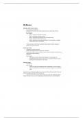
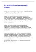
A histogram is a graph that shows the frequency of
‘specified’/groups of objects or subjects. A histogram looks like a
boxplot, the only difference is that a boxplot always has intervals of
1 on the X-axes while a histogram most often has a range on the X-
axes (though in theory 1’s could be possible as well I guess).
The graph to the left for example tells that there are around 5 trees
that have a height of 100-150cm, that there are 30 trees in between
150-200cm, around 26 in between a 200-250cm range and so on. In
this histogram you see that the range of a ‘defined’ height to count
for the amount is alternating with 50cm each time.
A histogram
1) uses quantitative data (quantitative data can be seen as values with numbers)
2) Has no gaps in between the ‘values’ (A graph with bars in this kind of sense is called a bar-graph;
bar graphs have categorical data, like names; but no numbers!), the only exception is when there is a
gap while there is no data (for example if there would be zero trees in between 200cm and 250cm)
3) The bar width (or Class/Bin size) is constant in a histogram (graph; 50cm width for each)
4) The Y-axis corresponds to the frequency (the frequency can be given as a ‘specific’ amount, but
also as a (relative) percentage)
When using brackets to make ‘groups of specific values’ (for example 200cm to 250cm) a bracket
means that the values gets included and parenthesis means that it not gets included (( [40,50); means
in some sort of way ‘ranging’ from 40 to 49; the 50 gets excluded (parenthesis), the 40 gets included
(brackets) ))
https://www.youtube.com/watch?v=sC7gjg9g3JU
, Statistics Intro; Median, Mean and Mode
Descriptive and inferential
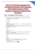
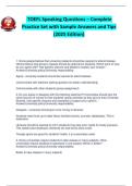
The average is a ‘typical’ or ‘middle’ number
of a series of values. You want to know/find
the central tendency.
- The Arithmetic Mean; The value
that is found when all combined values get
divided by the amount of values measured.
- The Median is the value that lies in
the middle of your values that are computed
in an ‘increasing’ value order (6,3,5,9,1;
1,3,5,6,9 Middle Number is 5; median is 5);
if the data set is an uneven amount of
number the middle number is the median, if
the data set exists out of an even amount of
values that the ‘arithmetic mean’ of the two
middle most values is the median.
- The Mode is the value that is found
in the highest frequency within a data set, if
there is no highest frequency of one specific
value then there is no mode.
https://www.youtube.com/watch?v=h8EYEJ32oQ8
Measures of dispersion; Range, variance and standard deviation
Population is the entire population of subjects and can be used to accurately calculate the values for
the population. A Sample on the other had is only a (random) part of the population and can only be
used to calculate an estimate of the values for the entire population; in reality the values for the
whole population will probably have somewhat different values, though in theory they should not
differ by a high amount.
In a lot of occasions the population mean of different data sets can be equal, even though the
disperse of the data sets highly alter; you could say that the disperse is the values in between the
means and the measured values.
For example; (1) -10, 0, 10, 20 and 30 And (2) 8, 9, 10, 11 and 12
Both have an arithmetic/population mean of 10
- The Range of a data set is simply the difference between the maximal and the minimal
measured value.
(1); Range = 30 - - 10 = 40
(2); Range = 12 – 8 = 4
- The Variance or σ2 (of a population data set) is the arithmetic mean of each value difference
in between the value and the arithmetic mean of the data set itself squared; ∑ (X −μ)2
N
NOIR; Nominal, Ordinal, Interval and Ratio
A Nominal measurement
has values that have no real
value; you can see the
numbers as 0 and 1 as
computer language, it’s
either false or true. But
while the numbers have no
real value almost nothing
can be measured with it
(except for example the
frequency of ‘0’ and ‘1’)
A nominal measurement for
example can be male and
female; here you can
understand that you cannot
measure a mean or median value of male and female.
Nominal can be split up into dichotomous
An Ordinal measurement has values that are not equal in each and every condition and where the
value ‘differences’ thus cannot be found equal. This means that you cannot say that someone’s pain
on a scale from 1 to 10 is double compared to someone else’s; you cannot know whether the change
between 4 and 5 is equal to the difference between 9 and 10. The ordinal measurements can have a 0
point, however this zero is arbitral; it is an idea and no exact/definitive zero.
An Interval measurement unlike an ordinal measurement has values that are concrete and whose
‘values differences’ are equal; for example on an exam the difference between 73 and 74 is equal to
the difference between 89 and 90. Interval measurements however still have an arbitrary zero value;
zero does not mean it is absent. For example temperature and test results; 0˚C does not mean that
there is no temperature, but interval measurements can also be negative. A test result on the other
hand can be 0, but that does not mean that a student has no knowledge (or brain).
The differences between adjacent values are always equal.
The Ratio measurements are measurements that can be used for each and every calculation, this
while the differences in between values are equal and while the zero value is exact; 0 means (Natural
Zero) that it is absent, negative values are impossible. For example height and weight; the differences
between 10kg and 11kg equal to the difference between 87kg and 88kg. Negative values do not exist,
you cannot be -2cm for example.
While the ratio measurements are exact and have a determined ‘0-value’ ratio measurements can be
used to define ‘multipliers’; for example someone who weighs 100kg weighs twice as much as
someone who weighs 50kg.
https://www.youtube.com/watch?v=LPHYPXBK_ks
,Discrete and Continuous Random Variables
Discrete random variables are limited in their exact values; discrete values can be counted and are
not infinite. You could say that discrete values are either an amount of things or values that are exact
to a certain degree; for example the amount of animals a zoo has, but also for example the time
rounded up to minutes. (As long as there are no infinite possibilities in between the values they are
discrete values)
Discrete values can also be ‘yes or no’ questions or multiple-choice in theory; there only are a certain
amount of possibilities the values can take up.
Continuous random variables can be much more precise than discrete random variables, but there
also lies the problem; the amount of possible values is infinite. A continuous random variable can in
theory take every value in between 0 and infinite; thus 7, 1.103 and 100.230, but also for example
0.234617 or 0.23461698.
Continuous random variables can for example be the exact time it is at any given time (exact here has
no ‘end’ definition in minutes; but in theory has no end). Continuous random variables in theory can
always be more precise.
https://www.youtube.com/watch?v=dOr0NKyD31Q
Histogram
A histogram is a graph that shows the frequency of
‘specified’/groups of objects or subjects. A histogram looks like a
boxplot, the only difference is that a boxplot always has intervals of
1 on the X-axes while a histogram most often has a range on the X-
axes (though in theory 1’s could be possible as well I guess).
The graph to the left for example tells that there are around 5 trees
that have a height of 100-150cm, that there are 30 trees in between
150-200cm, around 26 in between a 200-250cm range and so on. In
this histogram you see that the range of a ‘defined’ height to count
for the amount is alternating with 50cm each time.
A histogram
1) uses quantitative data (quantitative data can be seen as values with numbers)
2) Has no gaps in between the ‘values’ (A graph with bars in this kind of sense is called a bar-graph;
bar graphs have categorical data, like names; but no numbers!), the only exception is when there is a
gap while there is no data (for example if there would be zero trees in between 200cm and 250cm)
3) The bar width (or Class/Bin size) is constant in a histogram (graph; 50cm width for each)
4) The Y-axis corresponds to the frequency (the frequency can be given as a ‘specific’ amount, but
also as a (relative) percentage)
When using brackets to make ‘groups of specific values’ (for example 200cm to 250cm) a bracket
means that the values gets included and parenthesis means that it not gets included (( [40,50); means
in some sort of way ‘ranging’ from 40 to 49; the 50 gets excluded (parenthesis), the 40 gets included
(brackets) ))
https://www.youtube.com/watch?v=sC7gjg9g3JU
, Statistics Intro; Median, Mean and Mode
Descriptive and inferential
The average is a ‘typical’ or ‘middle’ number
of a series of values. You want to know/find
the central tendency.
- The Arithmetic Mean; The value
that is found when all combined values get
divided by the amount of values measured.
- The Median is the value that lies in
the middle of your values that are computed
in an ‘increasing’ value order (6,3,5,9,1;
1,3,5,6,9 Middle Number is 5; median is 5);
if the data set is an uneven amount of
number the middle number is the median, if
the data set exists out of an even amount of
values that the ‘arithmetic mean’ of the two
middle most values is the median.
- The Mode is the value that is found
in the highest frequency within a data set, if
there is no highest frequency of one specific
value then there is no mode.
https://www.youtube.com/watch?v=h8EYEJ32oQ8
Measures of dispersion; Range, variance and standard deviation
Population is the entire population of subjects and can be used to accurately calculate the values for
the population. A Sample on the other had is only a (random) part of the population and can only be
used to calculate an estimate of the values for the entire population; in reality the values for the
whole population will probably have somewhat different values, though in theory they should not
differ by a high amount.
In a lot of occasions the population mean of different data sets can be equal, even though the
disperse of the data sets highly alter; you could say that the disperse is the values in between the
means and the measured values.
For example; (1) -10, 0, 10, 20 and 30 And (2) 8, 9, 10, 11 and 12
Both have an arithmetic/population mean of 10
- The Range of a data set is simply the difference between the maximal and the minimal
measured value.
(1); Range = 30 - - 10 = 40
(2); Range = 12 – 8 = 4
- The Variance or σ2 (of a population data set) is the arithmetic mean of each value difference
in between the value and the arithmetic mean of the data set itself squared; ∑ (X −μ)2
N