May 6, 2020 APM346 – Week 2 Justin Ko
1 The Transport Equation
The transport equation models the concentration of a substance flowing in a fluid at a constant rate.
Definition 1. For parameters c ∈ R, the transport equation on R × R+ is
ut + cux = 0. (1)
The corresponding IVP for the transport equation is
(
ut + cux = 0 x ∈ R, t > 0
(2)
u|t=0 = f (x) x ∈ R.
The solution to this equation is derived using a method called the method of characteristics.
Theorem 1 (Solution to the Transport Equation)
(a) The general solution to (1) is
u(x, t) = φ(x − ct), (3)
where φ is an arbitrary function.
(b) The particular solution to (2) is
u(x, t) = f (x − ct). (4)
1.1 Derivation of the General Solution
We give two derivations of (3). Consider the general constant coefficient equation on R2
aux + buy = 0. (5)
1.1.1 Method 1: Integral Curves
We present a geometric derivation of general solution. If we define ~c = (a, b), then the (5) can be
written as
∇c u := ~c · ∇u = aux + buy = 0.
That is, the directional derivative of u in direction ~c is 0, so u is constant along the lines parallel to ~c.
y
x
Page 1 of 12
, May 6, 2020 APM346 – Week 2 Justin Ko
b
Notice that the vector ~c has corresponds to lines with slope a, so it described by the integral curves
satisfying the characteristic equations
dy b dx dy
= =⇒ = . (6)
dx a a b
b
The equations for lines with slope a can be recovered by integrating (6),
dx dy
= =⇒ ay = bx + C =⇒ ay − bx = C.
a b
Therefore, the solution only depends on the family of characteristic curves of the form ay − bx = C.
These lines can be parameterized by C, so
u(x, y) = φ(C) = φ(ay − bx)
for some function φ : R → R.
1.1.2 Method 2: Change of Variables
Using the characteristic equations
dx dy
= , (7)
a b
we can do a change of variables to reduce the PDE into an ODE. Integrating (7) implies
dx dy C + bx
= =⇒ ay = bx + C =⇒ ay − bx = C =⇒ y = .
a b a
We now treat y as a function of C and x and define
C + bx
v(x, C) := u(x, y(C, x)) where y(C, x) := .
a
By the multivariable chain rule,
∂ ∂ b
v(x, C) = ux + uy · y(C, x) = ux + uy · = 0.
∂x ∂x a
since u satisfies the equation (5). This is now an ODE in x, so we can integrate both sides with respect
to x to conclude that the general solution is of the form
v(x, C) = φ(C)
for some function φ : R → R. Since C = ay − bx and v(x, C) = u(x, y), we can write this equation
back in terms of u to conclude
u(x, y) = v(x, ay − bx) = φ(ay − bx).
Remark 1. We could’ve also written x as a function of y. If we did this, then we will have to treat
x as a function of C and y,
ay − C
x(C, y) = .
b
One can check that this choice of change of variables will give us the same solution.
Remark 2. One can check that Method 2 works even when a = 0 or b = 0 after a small modification.
Page 2 of 12
1 The Transport Equation
The transport equation models the concentration of a substance flowing in a fluid at a constant rate.
Definition 1. For parameters c ∈ R, the transport equation on R × R+ is
ut + cux = 0. (1)
The corresponding IVP for the transport equation is
(
ut + cux = 0 x ∈ R, t > 0
(2)
u|t=0 = f (x) x ∈ R.
The solution to this equation is derived using a method called the method of characteristics.
Theorem 1 (Solution to the Transport Equation)
(a) The general solution to (1) is
u(x, t) = φ(x − ct), (3)
where φ is an arbitrary function.
(b) The particular solution to (2) is
u(x, t) = f (x − ct). (4)
1.1 Derivation of the General Solution
We give two derivations of (3). Consider the general constant coefficient equation on R2
aux + buy = 0. (5)
1.1.1 Method 1: Integral Curves
We present a geometric derivation of general solution. If we define ~c = (a, b), then the (5) can be
written as
∇c u := ~c · ∇u = aux + buy = 0.
That is, the directional derivative of u in direction ~c is 0, so u is constant along the lines parallel to ~c.
y
x
Page 1 of 12
, May 6, 2020 APM346 – Week 2 Justin Ko
b
Notice that the vector ~c has corresponds to lines with slope a, so it described by the integral curves
satisfying the characteristic equations
dy b dx dy
= =⇒ = . (6)
dx a a b
b
The equations for lines with slope a can be recovered by integrating (6),
dx dy
= =⇒ ay = bx + C =⇒ ay − bx = C.
a b
Therefore, the solution only depends on the family of characteristic curves of the form ay − bx = C.
These lines can be parameterized by C, so
u(x, y) = φ(C) = φ(ay − bx)
for some function φ : R → R.
1.1.2 Method 2: Change of Variables
Using the characteristic equations
dx dy
= , (7)
a b
we can do a change of variables to reduce the PDE into an ODE. Integrating (7) implies
dx dy C + bx
= =⇒ ay = bx + C =⇒ ay − bx = C =⇒ y = .
a b a
We now treat y as a function of C and x and define
C + bx
v(x, C) := u(x, y(C, x)) where y(C, x) := .
a
By the multivariable chain rule,
∂ ∂ b
v(x, C) = ux + uy · y(C, x) = ux + uy · = 0.
∂x ∂x a
since u satisfies the equation (5). This is now an ODE in x, so we can integrate both sides with respect
to x to conclude that the general solution is of the form
v(x, C) = φ(C)
for some function φ : R → R. Since C = ay − bx and v(x, C) = u(x, y), we can write this equation
back in terms of u to conclude
u(x, y) = v(x, ay − bx) = φ(ay − bx).
Remark 1. We could’ve also written x as a function of y. If we did this, then we will have to treat
x as a function of C and y,
ay − C
x(C, y) = .
b
One can check that this choice of change of variables will give us the same solution.
Remark 2. One can check that Method 2 works even when a = 0 or b = 0 after a small modification.
Page 2 of 12