SOLUTIONS MANUAL
, TABLE OF CONTENTS
Solutions to Problems in Chapter 2 pp. 1-18
Solutions to Problems in Chapter 3 pp. 19-28
Solutions to Problems in Chapter 4 pp. 29-48
Solutions to Problems in Chapter 5 pp. 49-75
Solutions to Problems in Chapter 6 pp. 76-78
Solutions to Problems in Chapter 8 pp. 79-99
Solutions to Problems in Chapter 9 pp. 100-107
@
@SSeeisismmiciicsiiosolalatitoionn
, SOLUTIONS TO PROBLEMS IN CHAPTER 2
Problem 2.1. The results of tests to determine the modulus of rupture (MOR) for a set of timber
beams are shown in Table P2.1.
A. Plot the relative frequency and cumulative frequency histograms.
B. Calculate the sample mean, standard deviation, and coefficient of variation.
C. Plot the data on normal probability paper.
Solution:
A. For the histogram plots, the interval size is chosen to be 250. There are 45 data points.
Interval Relative Cumulative
Frequency Frequency
3250-3500 0 0
3500-3750 0.06667 0.066667
3750-4000 0.11111 0.177778
4000-4250 0.02222 0.200000
4250-4500 0.06667 0.266667
4500-4750 0.11111 0.377778
4750-5000 0.08889 0.466667
5000-5250 0.15556 0.622222
5250-5500 0.11111 0.733333
5500-5750 0.04444 0.777778
5750-6000 0.11111 0.888889
6000-6250 0.02222 0.911111
6250-6500 0.04444 0.955556
6500-6750 0 0.955556
6750-7000 0 0.955556
7000-7250 0.04444 1
7250-7500 0 1
Relative Frequency
0.18
0.16
0.14
0.12
0.1
0.08
0.06
0.04
0.02
0
3250-3500
3750-4000
4250-4500
4750-5000
5250-5500
5750-6000
6250-6500
6750-7000
7250-7500
@
@SSeeisismmiciicvsisoolalatitoionn
, Cumulative Frequency
1.2
1
0.8
0.6
0.4
0.2
0
3250-3500
3750-4000
4250-4500
4750-5000
5250-5500
5750-6000
6250-6500
6750-7000
7250-7500
B. Using Eqns. 2.25 and 2.26, sample mean = x = 5031 and sample standard deviation = sX =
880.4. The coefficient of variation based on sample parameters is sX / x = 0.175.
C. The step-by-step procedure described in Section 2.5 is followed to construct the plot on normal
probability paper.
MOR data on normal probability paper
3
Standard Normal Variate
2
1
0
-1
-2
-3
0 2000 4000 6000 8000
MOR
-------------------------------------------
Problem 2.2. A set of test data for the load-carrying capacity of a member is shown in Table P2.2.
A. Plot the test data on normal probability paper.
B. Plot a normal distribution on the same probability paper. Use the sample mean and
standard deviation as estimates of the true mean and standard deviation.
C. Plot a lognormal distribution on the same normal probability paper. Use the sample mean and
standard deviation as estimates of the true mean and standard deviation.
@
@SSeeisismmicicvisisoolalatitoionn
,D. Plot the relative frequency and cumulative frequency histograms.
Solution:
A. Using Eqns. 2.25 and 2.26, the sample mean, sample standard deviation, and sample
coefficient of variation are
x 4.127 s X 0.1770 CoV s X / x 0.04289
To plot on normal probability paper, we follow the step-by-step procedure outlined in Section 2.5.
-1
Raw Data Sorted i i/(N+1)=pi (pI)
3.95 3.74 1 0.05 -1.64485
4.07 3.90 2 0.10 -1.28155
4.14 3.95 3 0.15 -1.03643
3.99 3.97 4 0.20 -0.84162
4.21 3.99 5 0.25 -0.67449
4.39 4.04 6 0.30 -0.5244
4.21 4.05 7 0.35 -0.38532
3.90 4.07 8 0.40 -0.25335
3.74 4.07 9 0.45 -0.12566
4.28 4.14 10 0.50 0
4.15 4.15 11 0.55 0.125661
4.04 4.21 12 0.60 0.253347
4.26 4.21 13 0.65 0.385321
4.41 4.22 14 0.70 0.524401
4.22 4.26 15 0.75 0.67449
4.07 4.28 16 0.80 0.841621
3.97 4.36 17 0.85 1.036433
4.05 4.39 18 0.90 1.281551
4.36 4.41 19 0.95 1.644853
Normal Probability Paper
3
2
Standard Normal
1
0
Variate
3.5 3.7 3.9 4.1 4.3 4. 5
-1
-2
-3
Capacity
Raw data Normal Distribution
Lognormal distribution
@
@SSeeisismmicivcsiisoolalatitoionn
,B. See part A. To plot the normal distribution on normal probability paper: (1) Calculate values of
the standard normal variable z for some arbitrary values of x (in ascending order) in the range
of interest. The formula for z is
x x 4.127
z X
X
0.1770
(2) Plot z versus x on standard linear graph paper. The plot is shown in the graph in Part
A. Note that the relationship between z and x is linear, so only two points are needed to plot the
graph.
C. To plot a lognormal distribution, we need the lognormal distribution parameters. We will assume
that X= x and X=sX.
2 2 2
ln X ln(1 VX ) ln(1 (0.04289) ) ln X 0.04287
ln X ln( X ) 0.5 ln X ln(4.127) 0.5(0.04287)2 1.417
2
To plot the lognormal distribution on normal probability paper: (1) Calculate FX(x) for some arbitrary
values of x (in ascending order) in the range of interest. FX(x) is the lognormal distribution, and it
can be calculated as shown in Section 2.4.3. (2) Use the values of FX(xi) as the values of pi for
plotting points on normal probability paper. (3) Calculate zi = -1(pi). (4) Plot zi versus xi. The plot is
shown in the graph in Part A.
D. There are 19 data points. The interval size was chosen to be 0.05.
Interval Number Cumulative %
3.70-3.75 1 5.26%
3.75-3.8 0 5.26%
3.8-3.85 0 5.26%
3.85-3.9 1 10.53%
3.9-3.95 1 15.79%
3.95-4.0 2 26.32%
4.0-4.05 2 36.84%
4.05-4.1 2 47.37%
4.1-4.15 2 57.89%
4.15-4.2 0 57.89%
4.2-4.25 3 73.68%
4.25-4.3 2 84.21%
4.3-4.35 0 84.21%
4.35-4.4 2 94.74%
4.4-4.45 1 100.00%
@
@SSeeisismmicvicsiiosolalatitoionn
, Relative Frequency Plot
0.18
0.16
Relative frequency
0.14
0.12
0.1
0.08
0.06
0.04
0.02
0
3.8-3.85
3.9-3.95
4.0-4.05
4.1-4.15
4.2-4.25
4.3-4.35
4.4-4.45
3.70-3.75
Intervals
Cumulative Frequency Plot
100.00%
80.00%
60.00%
40.00%
20.00%
.00%
3.70-3.75
3.8-3.85
3.9-3.95
4.0-4.05
4.1-4.15
4.2-4.25
4.3-4.35
4.4-4.45
Intervals
--------------------------------------
Problem 2.3. For the data in Table 2.5, calculate the statistical estimate of the correlation coefficient
using Equation (2.99).
Solution:
The formula is
n
n
x i x yi y xi yi nxy
1 1
ˆ XY i1 i1
n 1 s Xs Y n 1 s Xs Y
Note that is doesn’t matter which variable is x and which is y. There are 100 data points. After
manipulating the data, you should find:
@
@SSeeisismmicviiicsiiosolalatitoionn
, for fc x 2743.82 s X 520.082
for E y 2991380 s Y 361245
ˆ XY 0.806
--------------------------------------------
Problem 2.4. A variable X is to be modelled using a uniform distribution. The lower bound value is 5,
and the upper bound value is 36.
A. Calculate the mean and standard deviation of X.
B. What is the probability that the value of X is between 10 and 20?
C. What is the probability that the value of X is greater than 31?
D. Plot the CDF on normal probability paper.
Solution:
A. The value of a is 5, and the value of b is 36. (Refer to Eqn. 2.31.) Using Eqns. 2.32 and
2.33,
a b
20.5
X
2
2
X 2 (b a) 80.1 8.95
X
12
B. Using Eqn. 2.31 and the definition of CDF (Eqn. 2.13),
x
1 1
FX (x) 5 d (x 5)
b a 31
Therefore, using Eqn. 2.15
15 5
P(10 x 20) FX (20) FX (10) 0.3226
31 31
C.
26
P(X 31) 1 P(X 31) 1 FX (31) 1 0.1613
31
D. To plot the uniform distribution on normal probability paper: (1) Calculate FX(x) for some arbitrary
values of x (in ascending order) in the range of interest. FX(x) is the uniform distribution, and
its range is limited. (2) Use the values of FX(xi) as the values of pi for plotting points on normal
probability paper. (3) Calculate zi = -1(pi). (4) Plot zi versus xi on standard linear graph paper
as shown below.
@
@SSeeisismmiciiicxsisoolalatitoionn
, Uniform distribution
3
Standard Normal Variable
2
1
0
0 10 20 30 40
-1
-2
-3
X
----------------------------------------
Problem 2.5. The dead load D on a structure is to be modelled as a normal random variable with a mean
value of 100 and a coefficient of variation of 8%.
A. Plot the PDF and CDF on standard graph paper.
B. Plot the CDF on normal probability paper.
C. Determine the probability that D is less than or equal to 95.
D. Determine the probability that D is between 95 and 105.
Solution:
A. The formulas for PDF and CDF are given by Eqns. 2.34 and 2.39. The value of D is VD D =
0.08(100)=8. Appendix B can be used to determine values of CDF, or a computer
spreadsheet program can be used.
PDF Function
0.06
0.05
0.04
PDF
0.03
0.02
0.01
0
70 80 90 100 110 120 130
x
, THOSE WERE PREVIEW PAGES
TO DOWNLOAD THE FULL PDF
CLICK ON THE L.I.N.K
ON THE NEXT PAGE
, TABLE OF CONTENTS
Solutions to Problems in Chapter 2 pp. 1-18
Solutions to Problems in Chapter 3 pp. 19-28
Solutions to Problems in Chapter 4 pp. 29-48
Solutions to Problems in Chapter 5 pp. 49-75
Solutions to Problems in Chapter 6 pp. 76-78
Solutions to Problems in Chapter 8 pp. 79-99
Solutions to Problems in Chapter 9 pp. 100-107
@
@SSeeisismmiciicsiiosolalatitoionn
, SOLUTIONS TO PROBLEMS IN CHAPTER 2
Problem 2.1. The results of tests to determine the modulus of rupture (MOR) for a set of timber
beams are shown in Table P2.1.
A. Plot the relative frequency and cumulative frequency histograms.
B. Calculate the sample mean, standard deviation, and coefficient of variation.
C. Plot the data on normal probability paper.
Solution:
A. For the histogram plots, the interval size is chosen to be 250. There are 45 data points.
Interval Relative Cumulative
Frequency Frequency
3250-3500 0 0
3500-3750 0.06667 0.066667
3750-4000 0.11111 0.177778
4000-4250 0.02222 0.200000
4250-4500 0.06667 0.266667
4500-4750 0.11111 0.377778
4750-5000 0.08889 0.466667
5000-5250 0.15556 0.622222
5250-5500 0.11111 0.733333
5500-5750 0.04444 0.777778
5750-6000 0.11111 0.888889
6000-6250 0.02222 0.911111
6250-6500 0.04444 0.955556
6500-6750 0 0.955556
6750-7000 0 0.955556
7000-7250 0.04444 1
7250-7500 0 1
Relative Frequency
0.18
0.16
0.14
0.12
0.1
0.08
0.06
0.04
0.02
0
3250-3500
3750-4000
4250-4500
4750-5000
5250-5500
5750-6000
6250-6500
6750-7000
7250-7500
@
@SSeeisismmiciicvsisoolalatitoionn
, Cumulative Frequency
1.2
1
0.8
0.6
0.4
0.2
0
3250-3500
3750-4000
4250-4500
4750-5000
5250-5500
5750-6000
6250-6500
6750-7000
7250-7500
B. Using Eqns. 2.25 and 2.26, sample mean = x = 5031 and sample standard deviation = sX =
880.4. The coefficient of variation based on sample parameters is sX / x = 0.175.
C. The step-by-step procedure described in Section 2.5 is followed to construct the plot on normal
probability paper.
MOR data on normal probability paper
3
Standard Normal Variate
2
1
0
-1
-2
-3
0 2000 4000 6000 8000
MOR
-------------------------------------------
Problem 2.2. A set of test data for the load-carrying capacity of a member is shown in Table P2.2.
A. Plot the test data on normal probability paper.
B. Plot a normal distribution on the same probability paper. Use the sample mean and
standard deviation as estimates of the true mean and standard deviation.
C. Plot a lognormal distribution on the same normal probability paper. Use the sample mean and
standard deviation as estimates of the true mean and standard deviation.
@
@SSeeisismmicicvisisoolalatitoionn
,D. Plot the relative frequency and cumulative frequency histograms.
Solution:
A. Using Eqns. 2.25 and 2.26, the sample mean, sample standard deviation, and sample
coefficient of variation are
x 4.127 s X 0.1770 CoV s X / x 0.04289
To plot on normal probability paper, we follow the step-by-step procedure outlined in Section 2.5.
-1
Raw Data Sorted i i/(N+1)=pi (pI)
3.95 3.74 1 0.05 -1.64485
4.07 3.90 2 0.10 -1.28155
4.14 3.95 3 0.15 -1.03643
3.99 3.97 4 0.20 -0.84162
4.21 3.99 5 0.25 -0.67449
4.39 4.04 6 0.30 -0.5244
4.21 4.05 7 0.35 -0.38532
3.90 4.07 8 0.40 -0.25335
3.74 4.07 9 0.45 -0.12566
4.28 4.14 10 0.50 0
4.15 4.15 11 0.55 0.125661
4.04 4.21 12 0.60 0.253347
4.26 4.21 13 0.65 0.385321
4.41 4.22 14 0.70 0.524401
4.22 4.26 15 0.75 0.67449
4.07 4.28 16 0.80 0.841621
3.97 4.36 17 0.85 1.036433
4.05 4.39 18 0.90 1.281551
4.36 4.41 19 0.95 1.644853
Normal Probability Paper
3
2
Standard Normal
1
0
Variate
3.5 3.7 3.9 4.1 4.3 4. 5
-1
-2
-3
Capacity
Raw data Normal Distribution
Lognormal distribution
@
@SSeeisismmicivcsiisoolalatitoionn
,B. See part A. To plot the normal distribution on normal probability paper: (1) Calculate values of
the standard normal variable z for some arbitrary values of x (in ascending order) in the range
of interest. The formula for z is
x x 4.127
z X
X
0.1770
(2) Plot z versus x on standard linear graph paper. The plot is shown in the graph in Part
A. Note that the relationship between z and x is linear, so only two points are needed to plot the
graph.
C. To plot a lognormal distribution, we need the lognormal distribution parameters. We will assume
that X= x and X=sX.
2 2 2
ln X ln(1 VX ) ln(1 (0.04289) ) ln X 0.04287
ln X ln( X ) 0.5 ln X ln(4.127) 0.5(0.04287)2 1.417
2
To plot the lognormal distribution on normal probability paper: (1) Calculate FX(x) for some arbitrary
values of x (in ascending order) in the range of interest. FX(x) is the lognormal distribution, and it
can be calculated as shown in Section 2.4.3. (2) Use the values of FX(xi) as the values of pi for
plotting points on normal probability paper. (3) Calculate zi = -1(pi). (4) Plot zi versus xi. The plot is
shown in the graph in Part A.
D. There are 19 data points. The interval size was chosen to be 0.05.
Interval Number Cumulative %
3.70-3.75 1 5.26%
3.75-3.8 0 5.26%
3.8-3.85 0 5.26%
3.85-3.9 1 10.53%
3.9-3.95 1 15.79%
3.95-4.0 2 26.32%
4.0-4.05 2 36.84%
4.05-4.1 2 47.37%
4.1-4.15 2 57.89%
4.15-4.2 0 57.89%
4.2-4.25 3 73.68%
4.25-4.3 2 84.21%
4.3-4.35 0 84.21%
4.35-4.4 2 94.74%
4.4-4.45 1 100.00%
@
@SSeeisismmicvicsiiosolalatitoionn
, Relative Frequency Plot
0.18
0.16
Relative frequency
0.14
0.12
0.1
0.08
0.06
0.04
0.02
0
3.8-3.85
3.9-3.95
4.0-4.05
4.1-4.15
4.2-4.25
4.3-4.35
4.4-4.45
3.70-3.75
Intervals
Cumulative Frequency Plot
100.00%
80.00%
60.00%
40.00%
20.00%
.00%
3.70-3.75
3.8-3.85
3.9-3.95
4.0-4.05
4.1-4.15
4.2-4.25
4.3-4.35
4.4-4.45
Intervals
--------------------------------------
Problem 2.3. For the data in Table 2.5, calculate the statistical estimate of the correlation coefficient
using Equation (2.99).
Solution:
The formula is
n
n
x i x yi y xi yi nxy
1 1
ˆ XY i1 i1
n 1 s Xs Y n 1 s Xs Y
Note that is doesn’t matter which variable is x and which is y. There are 100 data points. After
manipulating the data, you should find:
@
@SSeeisismmicviiicsiiosolalatitoionn
, for fc x 2743.82 s X 520.082
for E y 2991380 s Y 361245
ˆ XY 0.806
--------------------------------------------
Problem 2.4. A variable X is to be modelled using a uniform distribution. The lower bound value is 5,
and the upper bound value is 36.
A. Calculate the mean and standard deviation of X.
B. What is the probability that the value of X is between 10 and 20?
C. What is the probability that the value of X is greater than 31?
D. Plot the CDF on normal probability paper.
Solution:
A. The value of a is 5, and the value of b is 36. (Refer to Eqn. 2.31.) Using Eqns. 2.32 and
2.33,
a b
20.5
X
2
2
X 2 (b a) 80.1 8.95
X
12
B. Using Eqn. 2.31 and the definition of CDF (Eqn. 2.13),
x
1 1
FX (x) 5 d (x 5)
b a 31
Therefore, using Eqn. 2.15
15 5
P(10 x 20) FX (20) FX (10) 0.3226
31 31
C.
26
P(X 31) 1 P(X 31) 1 FX (31) 1 0.1613
31
D. To plot the uniform distribution on normal probability paper: (1) Calculate FX(x) for some arbitrary
values of x (in ascending order) in the range of interest. FX(x) is the uniform distribution, and
its range is limited. (2) Use the values of FX(xi) as the values of pi for plotting points on normal
probability paper. (3) Calculate zi = -1(pi). (4) Plot zi versus xi on standard linear graph paper
as shown below.
@
@SSeeisismmiciiicxsisoolalatitoionn
, Uniform distribution
3
Standard Normal Variable
2
1
0
0 10 20 30 40
-1
-2
-3
X
----------------------------------------
Problem 2.5. The dead load D on a structure is to be modelled as a normal random variable with a mean
value of 100 and a coefficient of variation of 8%.
A. Plot the PDF and CDF on standard graph paper.
B. Plot the CDF on normal probability paper.
C. Determine the probability that D is less than or equal to 95.
D. Determine the probability that D is between 95 and 105.
Solution:
A. The formulas for PDF and CDF are given by Eqns. 2.34 and 2.39. The value of D is VD D =
0.08(100)=8. Appendix B can be used to determine values of CDF, or a computer
spreadsheet program can be used.
PDF Function
0.06
0.05
0.04
0.03
0.02
0.01
0
70 80 90 100 110 120 130
x
, THOSE WERE PREVIEW PAGES
TO DOWNLOAD THE FULL PDF
CLICK ON THE L.I.N.K
ON THE NEXT PAGE