STAT4 – juni 2025 1
THE ONE-WAY ANOVA
= ANalysis Of VAriance, the statistical methodology to compare the means of two or more between-subjects
groups
- It uses variances to make inferences about the means
- It is kind of a generalization of the independent groups t-test we already know
- It is the basic method to analyze data from experiments and randomized control trials (RCT’s)
EXPLORATORY DATA ANALYSIS
Before undertaking any inferential statistics, you should always take a look at the data in various ways
- The most direct way is just to look at (a part of) the data matrix
- Visualize the data, e.g. histogram, boxplot, scatterplot
- Some data passes the interocular trauma test, meaning patterns in the data are so obvious that no further
statistical analysis is needed
2 TYPES OF VARIABLES
- 1 continuous variable: the dependent variable Y, so the outcome you're measuring (e.g. test scores, weight,
reaction time)
- 1 categorical variable: the independent variable X, so the factor (with 2 or more groups) you're comparing
(e.g. different diets, teaching methods, drug types)
NOTATION AND INTERPRETATION
𝑦𝑖𝑗 The score of person 𝑖 in condition 𝑗 (with 𝑖 = 1 to
𝑚𝑗 and 𝑗 = 1 to 𝑎)
𝑚𝑗 The total number of persons in condition 𝑗
- Because 𝑚𝑗 has an index 𝑗, it is assumed that
the number of persons across conditions do
not have to be equal, an unbalanced design
- If the 𝑚𝑗 ’s are equal, the design is balanced
𝑎 The total number of conditions or groups of the
levels of the factor
𝑎
The total number of participants
𝑛 = ∑ 𝑚𝑗
𝑗=1
𝑚𝑗
∑𝑖=1 𝑦𝑖𝑗 The sample average in condition 𝑗
𝑦̅𝑗 =
𝑚𝑗
𝑚𝑗 𝑚𝑗
∑𝑎
𝑗=1 ∑𝑖=1 𝑦𝑖𝑗 ∑𝑎
𝑗=1 ∑𝑖=1 𝑦𝑖𝑗
The grand sample average
𝑦̅ = =
∑𝑎
𝑗=1 𝑚𝑗 𝑛
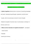
This data can be represented schematically in a table suitable for ANOVA >>
- Every row refers to one person and their score
- The columns refer to the variables
STATISTICAL INFERENCE FOR THE ANOVA MODEL
We want to answer the question whether there is a difference between the conditions AKA whether the
population means of the conditions differ
,STAT4 – juni 2025 2
1. MODELS AND HYPOTHESES
If you can translate a hypothesis into a statistical model, you can test the hypothesis using statistical methods
- The research question will be answered through a comparison of two (statistical) models: the full and the
reduced model, to see which one gets more support
- The models are so-called generative models because they specify completely how the scores on the
criterion variable are generated
THE FULL MODEL
𝑖𝑖𝑑
= 𝜇𝑗 + 𝜖𝑖𝑗 , where 𝜖𝑖𝑗 ∼ 𝑁(0, 𝜎 2 )
𝑦𝑖𝑗
- 𝜇𝑗 is the condition specific population mean
- 𝜖𝑖𝑗 is the random deviation/noise, assumed normal with mean 0 and variance 𝜎2
An observation 𝑦𝑖𝑗 can be decomposed in a systematic part (𝜇𝑗 ) and a random deviation (the stochastic 𝜖𝑖𝑗
or noise)
Since the population mean carries an index 𝑗, the population means are allowed to differ across conditions
THE REDUCED MODEL
𝑦𝑖𝑗 = 𝜇 + 𝜖𝑖𝑗
This is a special, less complex case of the full model that assumes that the 𝑎 means are all equal to each
other (𝜇1 = 𝜇2 = … = 𝜇a)
We see this restriction as the null hypothesis that is put to test: 𝐻0 : 𝜇1 = 𝜇2 = ⋯ = 𝜇𝑎
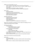
VISUAL ILLUSTRATION
Reduced model Full model
A table for the population means in the full and reduced model (for 𝑎 = 3) would look like this:
PARAMETER ESTIMATION
The population means in the full and reduced models are called parameters (𝜇 for reduced, 𝜇1 to 𝜇a for full)
- Parameters have a certain value in the population that is unknown to us, so we draw a sample from the
population, make observations and try to estimate the unknown population parameter
- In ANOVA, the standard method of estimation is the least squares estimation (Q), where you choose a value
for the parameters so that the sum of the squared differences between the observations and fitted values
(what the model proposes) are minimal
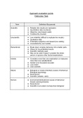
• For the reduced model:
,STAT4 – juni 2025 3
• For the full model:
• The residuals (difference between the observed score and the fitted value) will be the smallest (in
absolute value) under the full model as scores can lie closer to the data since it has more parameters
ERROR/RESIDUAL SUM OF SQUARES (SSE)
= measures the size of the residuals, and so the unexplained variability
- We again distinguish between the reduced and full model:
- The SSE is a measure of fit, and the smaller the 𝑆𝑆𝐸, the better the fit, as there will be less unexplained
variation
• It holds that 𝑆𝑆𝐸Reduced ≥ 𝑆𝑆𝐸Full
• In the full model, each condition gets its own mean, which allows a better fit since each condition's
data is centered around its own group mean
• In the reduced model, all conditions share the same 𝑦̅, and since we are forcing all observations to be
explained by a single mean, the fit is generally worse (or at best, the same)
- The effect sum of squares (SSEff) calculates the difference between the full and reduced model SSE’s,
expressing the variability explained by the model
• It is also called the between-group sum of squares
- Interpreting the magnitude of the SSE and SSEff is not straightforward
• The sum of squares are sensitive to scaling, so they cannot be interpreted meaningfully in an absolute
way, only relative to one another, e.g. multiplying all scores with 100 will increase the sum of squares
with 10000
• It is to be expected that when H0 is true, the effect sum of squares is relatively small, but what is small?
We need to take into account the complexity of the models and therefore the degrees of freedom!
DEGREES OF FREEDOM
Degrees of freedom (df) tell us how many values in our dataset are free to vary when estimating parameters
- df = number of observations – number of freely estimated parameters in the model
- If you have n numbers, and you know their average, then only (n - 1) of them are truly free to change
because the last number must be whatever makes the sum correct
- This "restriction" (or constraint) happens because we estimate parameters (like means), and those
estimations reduce the independent information in our dataset
- df play an important role as they determine the shape of the sampling distribution of the test statistic
IN THE REDUCED MODEL
In the reduced model, we assume there is only one mean (𝜇) for all groups, so:
- We have n data points (all observations across all conditions)
- But we estimated 1 parameter (𝜇, the overall mean)
- This means only (n - 1) data points are free to vary
𝑑𝑓𝑅𝑒𝑑𝑢𝑐𝑒𝑑 = ∑𝑎𝑗=1 𝑚𝑗 − 1 = 𝑛 − 1
, STAT4 – juni 2025 4
IN THE FULL MODEL
In the full model, we estimate one mean for each condition (𝜇1 to 𝜇a), so:
- We estimate a parameters (one per condition)
- Since we still have n total data points, but we've estimated a means, we have fewer free residuals
• The df for the full model will therefore always be lower than those for the reduced model!
𝑑𝑓𝑅𝑒𝑑𝑢𝑐𝑒𝑑 = ∑𝑎𝑗=1 𝑚𝑗 − 𝑎 = 𝑛 − 𝑎
DF FOR THE EFFECT
= how many independent pieces of information we have to estimate the effect of our categorical variable
= between-group degrees of freedom
𝑑𝑓𝐸𝑓𝑓 = 𝑑𝑓𝑅𝑒𝑑𝑢𝑐𝑒𝑑 − 𝑑𝑓𝐹𝑢𝑙𝑙 = (𝑛 − 1) − (𝑛 − 𝑎) = 𝑎 − 1
MEAN SQUARES
Dividing the sum of squares by their corresponding degrees of freedom gives the mean square (error):
𝑆𝑆𝐸
- 𝑀𝑆𝐸𝑅𝑒𝑑𝑢𝑐𝑒𝑑 = 𝑅𝑒𝑑𝑢𝑐𝑒𝑑 𝑛−1
𝑆𝑆𝐸 𝐹𝑢𝑙𝑙
- Mean square within groups / residuals: 𝑀𝑆𝐸𝐹𝑢𝑙𝑙 = 𝑛−𝑎
- It can also give the mean square effect by dividing the sum of squares by the difference between the
degrees of freedom of the reduced and full model
• 𝑑𝑓𝐸𝑓𝑓 = 𝑑𝑓𝑅𝑒𝑑𝑢𝑐𝑒𝑑 − 𝑑𝑓𝐹𝑢𝑙𝑙 = (𝑛 − 1) − (𝑛 − 𝑎) = 𝑎 − 1
𝑆𝑆𝐸𝑓𝑓
• 𝑀𝑆𝐸𝑓𝑓 = 𝑎−1
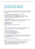
ALTERNATIVE PARAMETERIZATION
= another way of formulating the full model, because if the full model is defined as 𝑦𝑖𝑗 = 𝜇𝑗 + 𝜖𝑖𝑗 and the grand
1
population mean is the average of the condition specific population means 𝜇 = 𝑎 ∑𝑎𝑗=1 𝜇𝑗 , then we can rewrite
the full model:
- 𝛼j (≠ 𝑎!)is the effect parameter for group j, which expresses the effect or deviation of condition j compared
to the grand mean 𝜇
• It holds that summing all differences will always result in zero:
• The estimate of an effect parameter is calculated by subtracting the mean of the observations in group
1
j by the average of all group means: 𝛼̂𝑗 = 𝑦𝑗 − 𝑎 ∑𝑎𝑗=1 𝑦𝑗
- 𝜇 in this model is the grand average!
• In the reduced model, the best estimate for the mean is the mean of all observations: 𝜇̂ = 𝑦̅
• In the full model, the best estimate for the mean is the mean of all group means, so the grand average
1
which serves as a reference point for the group-specific means: 𝜇̂ = 𝑎 ∑𝑎𝑗=1 𝑦𝑗
• These 𝜇 match if the design is balanced (meaning each group has the same number of observations)
because all groups contribute equally
• These 𝜇 do not match if the design is unbalanced, since the reduced model (which uses the overall
mean) favors bigger groups, while the full model (which averages the group means) treats all groups
equally, leading to different results
THE ONE-WAY ANOVA
= ANalysis Of VAriance, the statistical methodology to compare the means of two or more between-subjects
groups
- It uses variances to make inferences about the means
- It is kind of a generalization of the independent groups t-test we already know
- It is the basic method to analyze data from experiments and randomized control trials (RCT’s)
EXPLORATORY DATA ANALYSIS
Before undertaking any inferential statistics, you should always take a look at the data in various ways
- The most direct way is just to look at (a part of) the data matrix
- Visualize the data, e.g. histogram, boxplot, scatterplot
- Some data passes the interocular trauma test, meaning patterns in the data are so obvious that no further
statistical analysis is needed
2 TYPES OF VARIABLES
- 1 continuous variable: the dependent variable Y, so the outcome you're measuring (e.g. test scores, weight,
reaction time)
- 1 categorical variable: the independent variable X, so the factor (with 2 or more groups) you're comparing
(e.g. different diets, teaching methods, drug types)
NOTATION AND INTERPRETATION
𝑦𝑖𝑗 The score of person 𝑖 in condition 𝑗 (with 𝑖 = 1 to
𝑚𝑗 and 𝑗 = 1 to 𝑎)
𝑚𝑗 The total number of persons in condition 𝑗
- Because 𝑚𝑗 has an index 𝑗, it is assumed that
the number of persons across conditions do
not have to be equal, an unbalanced design
- If the 𝑚𝑗 ’s are equal, the design is balanced
𝑎 The total number of conditions or groups of the
levels of the factor
𝑎
The total number of participants
𝑛 = ∑ 𝑚𝑗
𝑗=1
𝑚𝑗
∑𝑖=1 𝑦𝑖𝑗 The sample average in condition 𝑗
𝑦̅𝑗 =
𝑚𝑗
𝑚𝑗 𝑚𝑗
∑𝑎
𝑗=1 ∑𝑖=1 𝑦𝑖𝑗 ∑𝑎
𝑗=1 ∑𝑖=1 𝑦𝑖𝑗
The grand sample average
𝑦̅ = =
∑𝑎
𝑗=1 𝑚𝑗 𝑛
This data can be represented schematically in a table suitable for ANOVA >>
- Every row refers to one person and their score
- The columns refer to the variables
STATISTICAL INFERENCE FOR THE ANOVA MODEL
We want to answer the question whether there is a difference between the conditions AKA whether the
population means of the conditions differ
,STAT4 – juni 2025 2
1. MODELS AND HYPOTHESES
If you can translate a hypothesis into a statistical model, you can test the hypothesis using statistical methods
- The research question will be answered through a comparison of two (statistical) models: the full and the
reduced model, to see which one gets more support
- The models are so-called generative models because they specify completely how the scores on the
criterion variable are generated
THE FULL MODEL
𝑖𝑖𝑑
= 𝜇𝑗 + 𝜖𝑖𝑗 , where 𝜖𝑖𝑗 ∼ 𝑁(0, 𝜎 2 )
𝑦𝑖𝑗
- 𝜇𝑗 is the condition specific population mean
- 𝜖𝑖𝑗 is the random deviation/noise, assumed normal with mean 0 and variance 𝜎2
An observation 𝑦𝑖𝑗 can be decomposed in a systematic part (𝜇𝑗 ) and a random deviation (the stochastic 𝜖𝑖𝑗
or noise)
Since the population mean carries an index 𝑗, the population means are allowed to differ across conditions
THE REDUCED MODEL
𝑦𝑖𝑗 = 𝜇 + 𝜖𝑖𝑗
This is a special, less complex case of the full model that assumes that the 𝑎 means are all equal to each
other (𝜇1 = 𝜇2 = … = 𝜇a)
We see this restriction as the null hypothesis that is put to test: 𝐻0 : 𝜇1 = 𝜇2 = ⋯ = 𝜇𝑎
VISUAL ILLUSTRATION
Reduced model Full model
A table for the population means in the full and reduced model (for 𝑎 = 3) would look like this:
PARAMETER ESTIMATION
The population means in the full and reduced models are called parameters (𝜇 for reduced, 𝜇1 to 𝜇a for full)
- Parameters have a certain value in the population that is unknown to us, so we draw a sample from the
population, make observations and try to estimate the unknown population parameter
- In ANOVA, the standard method of estimation is the least squares estimation (Q), where you choose a value
for the parameters so that the sum of the squared differences between the observations and fitted values
(what the model proposes) are minimal
• For the reduced model:
,STAT4 – juni 2025 3
• For the full model:
• The residuals (difference between the observed score and the fitted value) will be the smallest (in
absolute value) under the full model as scores can lie closer to the data since it has more parameters
ERROR/RESIDUAL SUM OF SQUARES (SSE)
= measures the size of the residuals, and so the unexplained variability
- We again distinguish between the reduced and full model:
- The SSE is a measure of fit, and the smaller the 𝑆𝑆𝐸, the better the fit, as there will be less unexplained
variation
• It holds that 𝑆𝑆𝐸Reduced ≥ 𝑆𝑆𝐸Full
• In the full model, each condition gets its own mean, which allows a better fit since each condition's
data is centered around its own group mean
• In the reduced model, all conditions share the same 𝑦̅, and since we are forcing all observations to be
explained by a single mean, the fit is generally worse (or at best, the same)
- The effect sum of squares (SSEff) calculates the difference between the full and reduced model SSE’s,
expressing the variability explained by the model
• It is also called the between-group sum of squares
- Interpreting the magnitude of the SSE and SSEff is not straightforward
• The sum of squares are sensitive to scaling, so they cannot be interpreted meaningfully in an absolute
way, only relative to one another, e.g. multiplying all scores with 100 will increase the sum of squares
with 10000
• It is to be expected that when H0 is true, the effect sum of squares is relatively small, but what is small?
We need to take into account the complexity of the models and therefore the degrees of freedom!
DEGREES OF FREEDOM
Degrees of freedom (df) tell us how many values in our dataset are free to vary when estimating parameters
- df = number of observations – number of freely estimated parameters in the model
- If you have n numbers, and you know their average, then only (n - 1) of them are truly free to change
because the last number must be whatever makes the sum correct
- This "restriction" (or constraint) happens because we estimate parameters (like means), and those
estimations reduce the independent information in our dataset
- df play an important role as they determine the shape of the sampling distribution of the test statistic
IN THE REDUCED MODEL
In the reduced model, we assume there is only one mean (𝜇) for all groups, so:
- We have n data points (all observations across all conditions)
- But we estimated 1 parameter (𝜇, the overall mean)
- This means only (n - 1) data points are free to vary
𝑑𝑓𝑅𝑒𝑑𝑢𝑐𝑒𝑑 = ∑𝑎𝑗=1 𝑚𝑗 − 1 = 𝑛 − 1
, STAT4 – juni 2025 4
IN THE FULL MODEL
In the full model, we estimate one mean for each condition (𝜇1 to 𝜇a), so:
- We estimate a parameters (one per condition)
- Since we still have n total data points, but we've estimated a means, we have fewer free residuals
• The df for the full model will therefore always be lower than those for the reduced model!
𝑑𝑓𝑅𝑒𝑑𝑢𝑐𝑒𝑑 = ∑𝑎𝑗=1 𝑚𝑗 − 𝑎 = 𝑛 − 𝑎
DF FOR THE EFFECT
= how many independent pieces of information we have to estimate the effect of our categorical variable
= between-group degrees of freedom
𝑑𝑓𝐸𝑓𝑓 = 𝑑𝑓𝑅𝑒𝑑𝑢𝑐𝑒𝑑 − 𝑑𝑓𝐹𝑢𝑙𝑙 = (𝑛 − 1) − (𝑛 − 𝑎) = 𝑎 − 1
MEAN SQUARES
Dividing the sum of squares by their corresponding degrees of freedom gives the mean square (error):
𝑆𝑆𝐸
- 𝑀𝑆𝐸𝑅𝑒𝑑𝑢𝑐𝑒𝑑 = 𝑅𝑒𝑑𝑢𝑐𝑒𝑑 𝑛−1
𝑆𝑆𝐸 𝐹𝑢𝑙𝑙
- Mean square within groups / residuals: 𝑀𝑆𝐸𝐹𝑢𝑙𝑙 = 𝑛−𝑎
- It can also give the mean square effect by dividing the sum of squares by the difference between the
degrees of freedom of the reduced and full model
• 𝑑𝑓𝐸𝑓𝑓 = 𝑑𝑓𝑅𝑒𝑑𝑢𝑐𝑒𝑑 − 𝑑𝑓𝐹𝑢𝑙𝑙 = (𝑛 − 1) − (𝑛 − 𝑎) = 𝑎 − 1
𝑆𝑆𝐸𝑓𝑓
• 𝑀𝑆𝐸𝑓𝑓 = 𝑎−1
ALTERNATIVE PARAMETERIZATION
= another way of formulating the full model, because if the full model is defined as 𝑦𝑖𝑗 = 𝜇𝑗 + 𝜖𝑖𝑗 and the grand
1
population mean is the average of the condition specific population means 𝜇 = 𝑎 ∑𝑎𝑗=1 𝜇𝑗 , then we can rewrite
the full model:
- 𝛼j (≠ 𝑎!)is the effect parameter for group j, which expresses the effect or deviation of condition j compared
to the grand mean 𝜇
• It holds that summing all differences will always result in zero:
• The estimate of an effect parameter is calculated by subtracting the mean of the observations in group
1
j by the average of all group means: 𝛼̂𝑗 = 𝑦𝑗 − 𝑎 ∑𝑎𝑗=1 𝑦𝑗
- 𝜇 in this model is the grand average!
• In the reduced model, the best estimate for the mean is the mean of all observations: 𝜇̂ = 𝑦̅
• In the full model, the best estimate for the mean is the mean of all group means, so the grand average
1
which serves as a reference point for the group-specific means: 𝜇̂ = 𝑎 ∑𝑎𝑗=1 𝑦𝑗
• These 𝜇 match if the design is balanced (meaning each group has the same number of observations)
because all groups contribute equally
• These 𝜇 do not match if the design is unbalanced, since the reduced model (which uses the overall
mean) favors bigger groups, while the full model (which averages the group means) treats all groups
equally, leading to different results