Summary
Joya da Silva Patricio Gomes
Time Series Models
Email:
March 19, 2025
,Contents
Week 1 1
Time series . . . . . . . . . . . . . . . . . . . . . . . . . . . . . . . . . . . . . . . . . 1
Local Level Model . . . . . . . . . . . . . . . . . . . . . . . . . . . . . . . . . . . . . 1
Signal extraction: Kalman Filter . . . . . . . . . . . . . . . . . . . . . . . . . . . . . 2
Signal extraction: Kalman Smoother . . . . . . . . . . . . . . . . . . . . . . . . . . 4
Further inference . . . . . . . . . . . . . . . . . . . . . . . . . . . . . . . . . . . . . 5
Parameter estimation . . . . . . . . . . . . . . . . . . . . . . . . . . . . . . . . . . . 5
Week 2 7
Linear Gaussian Model . . . . . . . . . . . . . . . . . . . . . . . . . . . . . . . . . . 7
Examples . . . . . . . . . . . . . . . . . . . . . . . . . . . . . . . . . . . . . . . . . . 8
Lemmas . . . . . . . . . . . . . . . . . . . . . . . . . . . . . . . . . . . . . . . . . . 10
Kalman Filter and Proof . . . . . . . . . . . . . . . . . . . . . . . . . . . . . . . . . 10
Parameter estimation . . . . . . . . . . . . . . . . . . . . . . . . . . . . . . . . . . . 13
Further inference . . . . . . . . . . . . . . . . . . . . . . . . . . . . . . . . . . . . . 14
Week 3 15
Nonlinear functions . . . . . . . . . . . . . . . . . . . . . . . . . . . . . . . . . . . . 15
More Lemmas . . . . . . . . . . . . . . . . . . . . . . . . . . . . . . . . . . . . . . . 16
Simulation Smoothing . . . . . . . . . . . . . . . . . . . . . . . . . . . . . . . . . . 17
Nonlinear Models . . . . . . . . . . . . . . . . . . . . . . . . . . . . . . . . . . . . . 17
Stochastic Volatility Model . . . . . . . . . . . . . . . . . . . . . . . . . . . . . . . . 19
Quasi Maximum Likelihood . . . . . . . . . . . . . . . . . . . . . . . . . . . . . . . 19
Week 4 20
Nonlinear Non-Gaussian Models . . . . . . . . . . . . . . . . . . . . . . . . . . . . 20
Examples . . . . . . . . . . . . . . . . . . . . . . . . . . . . . . . . . . . . . . . . . . 20
Stacked Form Notation . . . . . . . . . . . . . . . . . . . . . . . . . . . . . . . . . . 22
Mode . . . . . . . . . . . . . . . . . . . . . . . . . . . . . . . . . . . . . . . . . . . . 23
Mode Estimation . . . . . . . . . . . . . . . . . . . . . . . . . . . . . . . . . . . . . 24
Importance Sampling . . . . . . . . . . . . . . . . . . . . . . . . . . . . . . . . . . . 26
Week 5 27
SPDK-Method . . . . . . . . . . . . . . . . . . . . . . . . . . . . . . . . . . . . . . . 27
MC-estimator . . . . . . . . . . . . . . . . . . . . . . . . . . . . . . . . . . . . . . . 28
Procedure . . . . . . . . . . . . . . . . . . . . . . . . . . . . . . . . . . . . . . . . . 29
Parameter Estimation . . . . . . . . . . . . . . . . . . . . . . . . . . . . . . . . . . . 30
Particle Filter . . . . . . . . . . . . . . . . . . . . . . . . . . . . . . . . . . . . . . . . 30
Bootstrap Filter . . . . . . . . . . . . . . . . . . . . . . . . . . . . . . . . . . . . . . 31
2
,Time Series Models Summary
Week 6 33
Multivariate Models . . . . . . . . . . . . . . . . . . . . . . . . . . . . . . . . . . . 33
Multivariate Local Level Model . . . . . . . . . . . . . . . . . . . . . . . . . . . . . 33
Multivariate Kalman Filter . . . . . . . . . . . . . . . . . . . . . . . . . . . . . . . . 35
Collapsing . . . . . . . . . . . . . . . . . . . . . . . . . . . . . . . . . . . . . . . . . 37
CONTENTS 3
, Week 1
Time series
A time series consists of n observations yt , ordered over time with index t = 1, . . . , n. If we
observe only one series over time, we refer to it as a univariate time series. If we observe
multiple series simultaneously, we refer to them as a multivariate time series (or panel
data). For example, let yit denote the homicide rate of country i in year t:
• Cross-sectional dimension indexed by i = 1, . . . , p (countries)
• Time-series dimension indexed by t = 1, . . . , n (years)
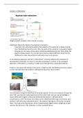
This means there are p · n observations in total. In time series, the part of the observation
that we aim to explain is called the signal and the noise is the part that remains unexplained.
The linear regression model (LRM) is
y t = Xt α + ϵt , ϵt ∼ N (0, σϵ2 ).
This can be expressed as
yt = signal + noise.
Estimation of the model using OLS and computation of the fitted values correspond to
extraction / estimation of signals.
Local Level Model
When data does not have any explanatory variables, we can try and estimate the constant
in the model
y t = α + ϵt .
Using OLS to estimate α will give us one constant level for the parameter while the level
might vary over time. In this case we try to model αt as a stochastic function over time:
α t +1 = α t + η t , ηt ∼ N (0, ση2 ).
Note that ηt is a random walk process (non-stationary). This makes the Local Level Model
(LLM):
y t = α t + ϵt ϵt ∼ N (0, σϵ2 )
α t +1 = α t + η t , ηt ∼ N (0, ση2 ),
where αt represents the state and ϵt the noise. The first equation is referred to as the obser-
vation equation (signal + noise). The second equation is called the state update equation.
In addition to these equations, we also need the initial condition α1 ∼ N ( a1 , P1 ). To account
1
Joya da Silva Patricio Gomes
Time Series Models
Email:
March 19, 2025
,Contents
Week 1 1
Time series . . . . . . . . . . . . . . . . . . . . . . . . . . . . . . . . . . . . . . . . . 1
Local Level Model . . . . . . . . . . . . . . . . . . . . . . . . . . . . . . . . . . . . . 1
Signal extraction: Kalman Filter . . . . . . . . . . . . . . . . . . . . . . . . . . . . . 2
Signal extraction: Kalman Smoother . . . . . . . . . . . . . . . . . . . . . . . . . . 4
Further inference . . . . . . . . . . . . . . . . . . . . . . . . . . . . . . . . . . . . . 5
Parameter estimation . . . . . . . . . . . . . . . . . . . . . . . . . . . . . . . . . . . 5
Week 2 7
Linear Gaussian Model . . . . . . . . . . . . . . . . . . . . . . . . . . . . . . . . . . 7
Examples . . . . . . . . . . . . . . . . . . . . . . . . . . . . . . . . . . . . . . . . . . 8
Lemmas . . . . . . . . . . . . . . . . . . . . . . . . . . . . . . . . . . . . . . . . . . 10
Kalman Filter and Proof . . . . . . . . . . . . . . . . . . . . . . . . . . . . . . . . . 10
Parameter estimation . . . . . . . . . . . . . . . . . . . . . . . . . . . . . . . . . . . 13
Further inference . . . . . . . . . . . . . . . . . . . . . . . . . . . . . . . . . . . . . 14
Week 3 15
Nonlinear functions . . . . . . . . . . . . . . . . . . . . . . . . . . . . . . . . . . . . 15
More Lemmas . . . . . . . . . . . . . . . . . . . . . . . . . . . . . . . . . . . . . . . 16
Simulation Smoothing . . . . . . . . . . . . . . . . . . . . . . . . . . . . . . . . . . 17
Nonlinear Models . . . . . . . . . . . . . . . . . . . . . . . . . . . . . . . . . . . . . 17
Stochastic Volatility Model . . . . . . . . . . . . . . . . . . . . . . . . . . . . . . . . 19
Quasi Maximum Likelihood . . . . . . . . . . . . . . . . . . . . . . . . . . . . . . . 19
Week 4 20
Nonlinear Non-Gaussian Models . . . . . . . . . . . . . . . . . . . . . . . . . . . . 20
Examples . . . . . . . . . . . . . . . . . . . . . . . . . . . . . . . . . . . . . . . . . . 20
Stacked Form Notation . . . . . . . . . . . . . . . . . . . . . . . . . . . . . . . . . . 22
Mode . . . . . . . . . . . . . . . . . . . . . . . . . . . . . . . . . . . . . . . . . . . . 23
Mode Estimation . . . . . . . . . . . . . . . . . . . . . . . . . . . . . . . . . . . . . 24
Importance Sampling . . . . . . . . . . . . . . . . . . . . . . . . . . . . . . . . . . . 26
Week 5 27
SPDK-Method . . . . . . . . . . . . . . . . . . . . . . . . . . . . . . . . . . . . . . . 27
MC-estimator . . . . . . . . . . . . . . . . . . . . . . . . . . . . . . . . . . . . . . . 28
Procedure . . . . . . . . . . . . . . . . . . . . . . . . . . . . . . . . . . . . . . . . . 29
Parameter Estimation . . . . . . . . . . . . . . . . . . . . . . . . . . . . . . . . . . . 30
Particle Filter . . . . . . . . . . . . . . . . . . . . . . . . . . . . . . . . . . . . . . . . 30
Bootstrap Filter . . . . . . . . . . . . . . . . . . . . . . . . . . . . . . . . . . . . . . 31
2
,Time Series Models Summary
Week 6 33
Multivariate Models . . . . . . . . . . . . . . . . . . . . . . . . . . . . . . . . . . . 33
Multivariate Local Level Model . . . . . . . . . . . . . . . . . . . . . . . . . . . . . 33
Multivariate Kalman Filter . . . . . . . . . . . . . . . . . . . . . . . . . . . . . . . . 35
Collapsing . . . . . . . . . . . . . . . . . . . . . . . . . . . . . . . . . . . . . . . . . 37
CONTENTS 3
, Week 1
Time series
A time series consists of n observations yt , ordered over time with index t = 1, . . . , n. If we
observe only one series over time, we refer to it as a univariate time series. If we observe
multiple series simultaneously, we refer to them as a multivariate time series (or panel
data). For example, let yit denote the homicide rate of country i in year t:
• Cross-sectional dimension indexed by i = 1, . . . , p (countries)
• Time-series dimension indexed by t = 1, . . . , n (years)
This means there are p · n observations in total. In time series, the part of the observation
that we aim to explain is called the signal and the noise is the part that remains unexplained.
The linear regression model (LRM) is
y t = Xt α + ϵt , ϵt ∼ N (0, σϵ2 ).
This can be expressed as
yt = signal + noise.
Estimation of the model using OLS and computation of the fitted values correspond to
extraction / estimation of signals.
Local Level Model
When data does not have any explanatory variables, we can try and estimate the constant
in the model
y t = α + ϵt .
Using OLS to estimate α will give us one constant level for the parameter while the level
might vary over time. In this case we try to model αt as a stochastic function over time:
α t +1 = α t + η t , ηt ∼ N (0, ση2 ).
Note that ηt is a random walk process (non-stationary). This makes the Local Level Model
(LLM):
y t = α t + ϵt ϵt ∼ N (0, σϵ2 )
α t +1 = α t + η t , ηt ∼ N (0, ση2 ),
where αt represents the state and ϵt the noise. The first equation is referred to as the obser-
vation equation (signal + noise). The second equation is called the state update equation.
In addition to these equations, we also need the initial condition α1 ∼ N ( a1 , P1 ). To account
1