MRM II NOTES
WEEK 1: Conceptual models & Analysis of Variance
What is a “model”?
- A simplified description of reality
- A visual representation of relations between theoretical constructs and variables
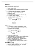
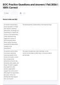
Moderating variable
- One variable moderates the relationship between two other variables
- It can either strengthen or weaken the existing relationship
- Communication skills moderate relationship between boring teacher and bored kids
- Provides nuance to research
- It is about change and about the relationship (interaction) between PVs
- The effect of one PV on the OV is moderated (depends on) another PV
- Can be positively or negatively moderating
- The moderator is only relevant if it happens together with the PV
- How sweet your coffee (OV) is depends on how much sugar you put in (PV)
moderated (MV) by how much you stir it
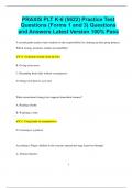
Mediating variable
- One variable mediates the relationship between the two other variables
- “Vehicle” variable: explains the relationship between the two other variables
- Slide quality mediates relationship between boring teacher and bored kids
- Some can be both mediating and moderating
How do you deal with multiple groups of data?
- We want to explain variability in the OV
- “Between groups” variability is identified as the variability explained by the model
- “Within groups” variability is variability not explained by the model
- ANOVA shows how group variability explains variability in the OV
- Comparing the means between groups shows “between group” variability
- ANOVA tests for the differences in the mean between groups
- ANOVA needs a quantitative OV and a categorical PV
- ANOVA decomposes total variance into variance explained by the model and
residual variance
ANOVA: (ANalysis Of VAriance)
- Compares the variability between groups with the variability within the groups
- How much of the outcome variable is explained by the predictor variable?
- Measurements of variability (how values differ in data) between groups
- Comparing differences between several means
, - Can go “one way” (one PV) or “two way” (more than one PV)
- ANOVA translates total variance into:
o Variance explained by the model
o Variance which is residual
How does ANOVA work?
- A one-way ANOVA can compare 2 (independent, “between-subject”) groups
- How much of the variability in our outcome is explained by our PV?
- Compares the variability between the groups against the variability within the groups
- Some variability can be explained by the PV
- But there is always residual variability that is unexplained
- ANOVA breaks down different measures of variability with sums of squares
- Helps us test if the mean scores of the groups are statistically different
ANOVA assumptions:
- When the OV is Quantitative
- When the PV is Categorical
- When there are more than 2 groups of PVs
- When variance is homogenous across groups
- When residuals are normally distributed
- When groups are roughly equally sized
- When data is “between subjects” (subjects can only be in one group at a time)
How to check for “homogeneity of variances”? = Levene’s test!
1) Find the table “Test of homogeneity of Variances”
2) Check the “sig”
a. Higher than 0.05? = group means homogenous, ANOVA can proceed
b. Significance? = group means heterogeneous, ANOVA can’t proceed
ANOVA Hypothesis:
H0 = no difference in μ’s between groups (μ1 = μ2 = μ3…)
H1 = at least two group μ’s are different (μ1 ≠ μ2 ≠ μ3…)
Conclusion: If the p < .05, then there is a statistically significant difference between at least
two of the group means and we reject the H0.
,ANOVA 1: calculate SST, the Total Sum of Squares
The step to take before you can run an ANOVA test:
- To find the total amount of variation within data, we calculate the difference between
each observed data point and the grand mean (Grand Mean = ybar = ȳ)
- Simplest model to fit a set of data: the mean of the PV and OV
- Square the differences, add them up = SST (Sum of Squares) (or Grand Variance)
- s2 (variance) = SS (Sum of Squares) ÷ (N – 1)
- SS = s2 x (N – 1)
Calculate the SST:
1) Start with the observed scores
2) Find the mean of all observed scores
3) Subtract observed means from grand mean (y - ȳ)
4) Square the result (y - ȳ)2
5) Add up everything Σ (y - ȳ)2
6) Multiply each result by the number of participants (“n”) Σn (y - ȳ)2
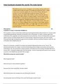
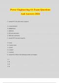
Sum of Squares formula:
Sum of Squares does not explain variance within each group; for this we need “residual”
ANOVA 2: Calculate the Sum of Squares “Between” and the Sum of Squares “Within”
- How much of the total variance is found between the total means of group 1
compared with group 2, compared with group 3 etc? = MODEL
- How much is found within group 1 or within group 2 etc? = RESIDUAL
What is “analysis of variance”?
- For a key outcome variable which is quantitative, we want to understand the spread
- High variance = broad range of responses, inconsistent values
- Low variance = narrow range of responses, scores that are similar to each other
Sum of Squares
- The Total Sum of Squares is the total variance across all groups (between-groups)
- Total Sum of Squares (SST) is made up of the Model Sum of Squares (SSM) and
Residual Sum of Squares (SSR)
o SSM explains variation between the various groups, explained by the model
o A low SSM means the model is a good fit
o An SSM of “0” means that there is no difference in the means of all groups
(but there can be high variability within the groups themselves)
o SSR explains other, random, unexplained variation
SStotal = SSmodel + SSresidual
Residual Sum of Squares = RSS or SSR
- How much of the variation cannot be explained by the model?
- What is the amount of “random” variation in the sample (individual height, weight)?
- What is the difference between what the model predicts and what was actually
observed?
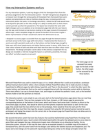
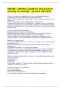
SSR = Σ (SSGROUP 1 + SSGROUP 2 + SSGROUP 3…)2
, SSR = Σ (VAREACHGROUP) x (n-1)
We come out with a percentage score:
If the SSR = 0%, then all groups have the same mean: our model, that PV influences
OV, means nothing
This means 95% of the variability within scores is due to the PV
“factor” is a PV
“levels” are PV categories (groups)
ANOVA in SPSS
F-Ratio
- F-ratio measures the improvement due to fitting the model
- Compares the group means versus the grand mean of scores for all participants
- Compares this against the error remaining in the model, which is the difference
between the actual scores and the respective means of the groups
- Ratio of explained variance relative to unexplained variance
- How good a test model is compared to the error within that model
- Divide the model mean squares (MSM) by the residual means square (MRR)
- If the value is less than 1, the effect is non-significant
- A good model has a large F-Ratio (greater than 1) because the “model” should be
larger than the “error”
F = MSM or systematic variation
MSR unsystematic variation
FRATIO = explained variability = between group variability
unexplained variability within group variability
WEEK 1: Conceptual models & Analysis of Variance
What is a “model”?
- A simplified description of reality
- A visual representation of relations between theoretical constructs and variables
Moderating variable
- One variable moderates the relationship between two other variables
- It can either strengthen or weaken the existing relationship
- Communication skills moderate relationship between boring teacher and bored kids
- Provides nuance to research
- It is about change and about the relationship (interaction) between PVs
- The effect of one PV on the OV is moderated (depends on) another PV
- Can be positively or negatively moderating
- The moderator is only relevant if it happens together with the PV
- How sweet your coffee (OV) is depends on how much sugar you put in (PV)
moderated (MV) by how much you stir it
Mediating variable
- One variable mediates the relationship between the two other variables
- “Vehicle” variable: explains the relationship between the two other variables
- Slide quality mediates relationship between boring teacher and bored kids
- Some can be both mediating and moderating
How do you deal with multiple groups of data?
- We want to explain variability in the OV
- “Between groups” variability is identified as the variability explained by the model
- “Within groups” variability is variability not explained by the model
- ANOVA shows how group variability explains variability in the OV
- Comparing the means between groups shows “between group” variability
- ANOVA tests for the differences in the mean between groups
- ANOVA needs a quantitative OV and a categorical PV
- ANOVA decomposes total variance into variance explained by the model and
residual variance
ANOVA: (ANalysis Of VAriance)
- Compares the variability between groups with the variability within the groups
- How much of the outcome variable is explained by the predictor variable?
- Measurements of variability (how values differ in data) between groups
- Comparing differences between several means
, - Can go “one way” (one PV) or “two way” (more than one PV)
- ANOVA translates total variance into:
o Variance explained by the model
o Variance which is residual
How does ANOVA work?
- A one-way ANOVA can compare 2 (independent, “between-subject”) groups
- How much of the variability in our outcome is explained by our PV?
- Compares the variability between the groups against the variability within the groups
- Some variability can be explained by the PV
- But there is always residual variability that is unexplained
- ANOVA breaks down different measures of variability with sums of squares
- Helps us test if the mean scores of the groups are statistically different
ANOVA assumptions:
- When the OV is Quantitative
- When the PV is Categorical
- When there are more than 2 groups of PVs
- When variance is homogenous across groups
- When residuals are normally distributed
- When groups are roughly equally sized
- When data is “between subjects” (subjects can only be in one group at a time)
How to check for “homogeneity of variances”? = Levene’s test!
1) Find the table “Test of homogeneity of Variances”
2) Check the “sig”
a. Higher than 0.05? = group means homogenous, ANOVA can proceed
b. Significance? = group means heterogeneous, ANOVA can’t proceed
ANOVA Hypothesis:
H0 = no difference in μ’s between groups (μ1 = μ2 = μ3…)
H1 = at least two group μ’s are different (μ1 ≠ μ2 ≠ μ3…)
Conclusion: If the p < .05, then there is a statistically significant difference between at least
two of the group means and we reject the H0.
,ANOVA 1: calculate SST, the Total Sum of Squares
The step to take before you can run an ANOVA test:
- To find the total amount of variation within data, we calculate the difference between
each observed data point and the grand mean (Grand Mean = ybar = ȳ)
- Simplest model to fit a set of data: the mean of the PV and OV
- Square the differences, add them up = SST (Sum of Squares) (or Grand Variance)
- s2 (variance) = SS (Sum of Squares) ÷ (N – 1)
- SS = s2 x (N – 1)
Calculate the SST:
1) Start with the observed scores
2) Find the mean of all observed scores
3) Subtract observed means from grand mean (y - ȳ)
4) Square the result (y - ȳ)2
5) Add up everything Σ (y - ȳ)2
6) Multiply each result by the number of participants (“n”) Σn (y - ȳ)2
Sum of Squares formula:
Sum of Squares does not explain variance within each group; for this we need “residual”
ANOVA 2: Calculate the Sum of Squares “Between” and the Sum of Squares “Within”
- How much of the total variance is found between the total means of group 1
compared with group 2, compared with group 3 etc? = MODEL
- How much is found within group 1 or within group 2 etc? = RESIDUAL
What is “analysis of variance”?
- For a key outcome variable which is quantitative, we want to understand the spread
- High variance = broad range of responses, inconsistent values
- Low variance = narrow range of responses, scores that are similar to each other
Sum of Squares
- The Total Sum of Squares is the total variance across all groups (between-groups)
- Total Sum of Squares (SST) is made up of the Model Sum of Squares (SSM) and
Residual Sum of Squares (SSR)
o SSM explains variation between the various groups, explained by the model
o A low SSM means the model is a good fit
o An SSM of “0” means that there is no difference in the means of all groups
(but there can be high variability within the groups themselves)
o SSR explains other, random, unexplained variation
SStotal = SSmodel + SSresidual
Residual Sum of Squares = RSS or SSR
- How much of the variation cannot be explained by the model?
- What is the amount of “random” variation in the sample (individual height, weight)?
- What is the difference between what the model predicts and what was actually
observed?
SSR = Σ (SSGROUP 1 + SSGROUP 2 + SSGROUP 3…)2
, SSR = Σ (VAREACHGROUP) x (n-1)
We come out with a percentage score:
If the SSR = 0%, then all groups have the same mean: our model, that PV influences
OV, means nothing
This means 95% of the variability within scores is due to the PV
“factor” is a PV
“levels” are PV categories (groups)
ANOVA in SPSS
F-Ratio
- F-ratio measures the improvement due to fitting the model
- Compares the group means versus the grand mean of scores for all participants
- Compares this against the error remaining in the model, which is the difference
between the actual scores and the respective means of the groups
- Ratio of explained variance relative to unexplained variance
- How good a test model is compared to the error within that model
- Divide the model mean squares (MSM) by the residual means square (MRR)
- If the value is less than 1, the effect is non-significant
- A good model has a large F-Ratio (greater than 1) because the “model” should be
larger than the “error”
F = MSM or systematic variation
MSR unsystematic variation
FRATIO = explained variability = between group variability
unexplained variability within group variability