Solutions Manual
Module A: Linear Programming
1. Maximum occurs at S = 1.333, T = 3.333, Profit = $50.67
Cognitive Domain: Knowledge
Difficulty Level: Easy
2a. The optimum solution occurs at X = 2, Y = 9 for Profit = $57.
2b. The constraints have zero slack; the solution lies at the intersection of these two
constraints. This means all 24 hours of fabrication time and 40 hours of assembly time are
used up when producing 2 of Y and 9 of Y to achieve a maximum profit of $57.
Cognitive Domain: Knowledge
Difficulty Level: Easy
3.
The optimal solution is X1 = 4.2, X2 = 1.6 for Cost = $26.4.
Cognitive Domain: Knowledge
Difficulty Level: Easy
,4a. Costs are minimized at 76 when P = 8 and R = 20.
4b. The third constraint has a surplus of 46, and the fourth constraint has a surplus of 15.
This means mixing 8 ounces of P and 20 ounces of R to obtain the lowest costs of $76; the
resulting mixture exceeds the protein requirement by 46 units and the amount of R
required by 15 units. Similarly, surplus is the amount by which the left-hand side values are
greater than the right-hand side values. So for the fourth constraint, R must be greater than
or equal to 5, but at the optimal solution R = 20, which is 15 greater than the constraint’s
RHS.
Cognitive Domain: Comprehension
Difficulty Level: Medium
5a. The optimal product mix is 925 soft, 150 hardwood, 200 tropical, and 300 aircraft for a
total profit of $21,800.
5b. The allowance increase and allowance decrease values for the objective function
coefficients define the range within which the unit profit of each types of plywood can
change without affecting the optimal profit of $21,800. For example, the allowance increase
and allowance decrease for soft plywood is infinity and 2, respectively. This means as long
as the unit profit for plywood is within the range of infinity to ($8 – $2) $6, the optimal
profit for Diamond Plywood stays at $21,800. Similarly, the optimal profit will stay at
$21,800 as long as the unit profit for hardwood is within the range of $0 to $20 ($12 + 8);
for tropical is $0 to $28 ($18 + 10); and for aircraft is $0 to $40 ($30 + 10).
5c. The shadow price of a constraint defines the increase/decrease in profit per unit
increase/decrease of that constraint’s RHS, as long as the change in the constraint’s RHS is
within the allowable increase/decrease. For example, the shadow price for grading time is
$8 with an allowance increase/decrease of 275 and 805. This means there will be an
increase of profit by $8 with an additional hour of grading time up to 275 hours (i.e., from
3,500 to 3,775 hours), and there will be a decrease of profit by $8, with each reduction of
grading time down to 805 hours (i.e., from 3,500 to 2,695 hours).
Cognitive Domain: Analysis
Difficulty Level: Medium
6a. Regular Blend should be made from 36 pounds of Hawaiian and 84 pounds of Ethiopian,
and Premium Blend should be made of 45 pounds Hawaiian, 25 pounds Ethiopian, and 30
pounds Columbian.
6b. The coefficients for Ethiopian Premium, Columbian Premium, and Columbian Regular all
show allowable decreases of infinity, meaning that their profit contributions could become
negative, yet they would still appear in the solution. While unprofitable, they are required in
order to achieve the required percentages in the various blends. The remainder of the
allowable increases and decreases show the range in which the coefficients must remain in
order to retain this optimal solution.
6c. Shadow prices are the marginal values for one additional unit of the right-hand side. The
shadow price for Columbian Premium is -2; if the RHS of the original constraint is increased
,by 1 unit, the value of the objective function at optimality drops by 2 units (in this case,
profits) as long as that increase or decrease is within plus 20 or minus 30 (the allowable
increase and decrease respectively). Changes in RHS values outside the allowable increases
and decreases will not be a direct multiplier of the shadow prices.
Cognitive Domain: Analysis
Difficulty Level: Medium
7a. The optimal schedule is as follows:
Workers Starting This
Time Interval
Shift
00–04 7
04–08 1
08–12 21
12–16 6
16–20 12
20–24 0
Based on this system of equations,
Min Z = x1 + x2 + x3 + x4 + x5 + x6
subject to :
x1 + x2 8
x2 + x3 22
x3 + x4 26
x4 + x5 18
x5 + x6 12
x6 + x1 7
7b. The allowable increase and decrease values for the objective function coefficients
provide a valid range for the reduced cost entries. In the objective function, all coefficients
are 1; counting the number of workers for any shift more than twice will result in a different
schedule but identical number of workers.
7c. Shadow prices are the marginal values for one additional unit of the right-hand side. If
the RHS of the original constraint is increased by 1 unit, the value of the objective function
at optimality changes by the value of the shadow price as long as that increase or decrease
is within the allowable increase and decrease. Changes in RHS values outside the allowable
increases and decreases will not be a direct multiplier of the shadow prices.
Cognitive Domain: Application
Difficulty Level: Hard
8.
Max Profit = $800W + $600R
subject to:
400W + 200 R ≤ 3200
, 2W + 3R ≤ 24
W + R ≤ 20
W + R ≥ 10
The optimal solution is 10W and 0R.
Cognitive Domain: Application
Difficulty Level: Hard
9a.
Max Z = 3P + 4 N
subject to :
P+N 4
16 P + 8 N 64
−2 P + N 0
9b.
Module A: Linear Programming
1. Maximum occurs at S = 1.333, T = 3.333, Profit = $50.67
Cognitive Domain: Knowledge
Difficulty Level: Easy
2a. The optimum solution occurs at X = 2, Y = 9 for Profit = $57.
2b. The constraints have zero slack; the solution lies at the intersection of these two
constraints. This means all 24 hours of fabrication time and 40 hours of assembly time are
used up when producing 2 of Y and 9 of Y to achieve a maximum profit of $57.
Cognitive Domain: Knowledge
Difficulty Level: Easy
3.
The optimal solution is X1 = 4.2, X2 = 1.6 for Cost = $26.4.
Cognitive Domain: Knowledge
Difficulty Level: Easy
,4a. Costs are minimized at 76 when P = 8 and R = 20.
4b. The third constraint has a surplus of 46, and the fourth constraint has a surplus of 15.
This means mixing 8 ounces of P and 20 ounces of R to obtain the lowest costs of $76; the
resulting mixture exceeds the protein requirement by 46 units and the amount of R
required by 15 units. Similarly, surplus is the amount by which the left-hand side values are
greater than the right-hand side values. So for the fourth constraint, R must be greater than
or equal to 5, but at the optimal solution R = 20, which is 15 greater than the constraint’s
RHS.
Cognitive Domain: Comprehension
Difficulty Level: Medium
5a. The optimal product mix is 925 soft, 150 hardwood, 200 tropical, and 300 aircraft for a
total profit of $21,800.
5b. The allowance increase and allowance decrease values for the objective function
coefficients define the range within which the unit profit of each types of plywood can
change without affecting the optimal profit of $21,800. For example, the allowance increase
and allowance decrease for soft plywood is infinity and 2, respectively. This means as long
as the unit profit for plywood is within the range of infinity to ($8 – $2) $6, the optimal
profit for Diamond Plywood stays at $21,800. Similarly, the optimal profit will stay at
$21,800 as long as the unit profit for hardwood is within the range of $0 to $20 ($12 + 8);
for tropical is $0 to $28 ($18 + 10); and for aircraft is $0 to $40 ($30 + 10).
5c. The shadow price of a constraint defines the increase/decrease in profit per unit
increase/decrease of that constraint’s RHS, as long as the change in the constraint’s RHS is
within the allowable increase/decrease. For example, the shadow price for grading time is
$8 with an allowance increase/decrease of 275 and 805. This means there will be an
increase of profit by $8 with an additional hour of grading time up to 275 hours (i.e., from
3,500 to 3,775 hours), and there will be a decrease of profit by $8, with each reduction of
grading time down to 805 hours (i.e., from 3,500 to 2,695 hours).
Cognitive Domain: Analysis
Difficulty Level: Medium
6a. Regular Blend should be made from 36 pounds of Hawaiian and 84 pounds of Ethiopian,
and Premium Blend should be made of 45 pounds Hawaiian, 25 pounds Ethiopian, and 30
pounds Columbian.
6b. The coefficients for Ethiopian Premium, Columbian Premium, and Columbian Regular all
show allowable decreases of infinity, meaning that their profit contributions could become
negative, yet they would still appear in the solution. While unprofitable, they are required in
order to achieve the required percentages in the various blends. The remainder of the
allowable increases and decreases show the range in which the coefficients must remain in
order to retain this optimal solution.
6c. Shadow prices are the marginal values for one additional unit of the right-hand side. The
shadow price for Columbian Premium is -2; if the RHS of the original constraint is increased
,by 1 unit, the value of the objective function at optimality drops by 2 units (in this case,
profits) as long as that increase or decrease is within plus 20 or minus 30 (the allowable
increase and decrease respectively). Changes in RHS values outside the allowable increases
and decreases will not be a direct multiplier of the shadow prices.
Cognitive Domain: Analysis
Difficulty Level: Medium
7a. The optimal schedule is as follows:
Workers Starting This
Time Interval
Shift
00–04 7
04–08 1
08–12 21
12–16 6
16–20 12
20–24 0
Based on this system of equations,
Min Z = x1 + x2 + x3 + x4 + x5 + x6
subject to :
x1 + x2 8
x2 + x3 22
x3 + x4 26
x4 + x5 18
x5 + x6 12
x6 + x1 7
7b. The allowable increase and decrease values for the objective function coefficients
provide a valid range for the reduced cost entries. In the objective function, all coefficients
are 1; counting the number of workers for any shift more than twice will result in a different
schedule but identical number of workers.
7c. Shadow prices are the marginal values for one additional unit of the right-hand side. If
the RHS of the original constraint is increased by 1 unit, the value of the objective function
at optimality changes by the value of the shadow price as long as that increase or decrease
is within the allowable increase and decrease. Changes in RHS values outside the allowable
increases and decreases will not be a direct multiplier of the shadow prices.
Cognitive Domain: Application
Difficulty Level: Hard
8.
Max Profit = $800W + $600R
subject to:
400W + 200 R ≤ 3200
, 2W + 3R ≤ 24
W + R ≤ 20
W + R ≥ 10
The optimal solution is 10W and 0R.
Cognitive Domain: Application
Difficulty Level: Hard
9a.
Max Z = 3P + 4 N
subject to :
P+N 4
16 P + 8 N 64
−2 P + N 0
9b.