Lecture 1: introduction to asset pricing + intertemporal choice and financial markets
Time and risk
Asset pricing = how to price a financial asset -> what is the theoretically correct price for an
asset?
Two important points:
- Prices are the mirror image of returns: high price, low return
- Price and value do not always coincide (not equal when there is mispricing)
To value an asset, we consider two components:
- time = the money you want for giving up liquidity (delay of payments)
- risk = chance that you get your money back (volatility of payments)
-> time is simple to account for, risk is not
On average, stock return are 9%:
-> 8% premium earned for holding risk -> more impactful
-> 1% premium due to interest rates
Asset pricing focuses more on pricing risk
Normative vs positive
In economics, there is a tension between positive and normative models:
- normative = we prescribe a choice, how things should be theoretically (prescriptive)
- positive = what people actually do with their choices (descriptive)
Joint hypothesis problem = you can make a judgement call on mispricing only if you have a
model that works which gives you a reference point (true fundamental value). You do not
know if your model is correct and your choice depends on the validity of the model. We
should always take theory with a grinch of salt.
This interpretation shapes not only our understanding of markets, but also our investment
strategies. If there is a mispricing, it is theoretically possible to make money off it. However,
this is not obvious. Example:
-> company is worth more/less and we want to make money out of this when it returns to
fundamental value. Even if you are right, but a lot of people trade in the other direction, you
can still lose money (GameStop).
If the world does not obey the model’s predictions, this opens up 2 possibilities.
- the model is wrong and needs improvement
- the world is wrong (mispricing)
Absolute vs relative
Asset pricing models can also be classified as absolute and relative:
- absolute = we price the theoretical price of each asset by reference to its exposure to
fundamental sources of macroeconomic risk (= systematic risk)
- relative = we determine the asset’s value by using the price of another asset as a
reference point (e.g. options). We do not evaluate if the other asset is mispriced or
where the price of the other asset came from. We basically ignore risk factors.
1
,We will work with absolute consumption-based models, where:
- the trade off between current and future consumption determines investments
- investments matter to the degree that they allow investors to smooth consumption
(constant consumption over time)
The absolute approach has its limits. The CAPM for instance is a bit of a hybrid:
- the market portfolio is the main determinant of asset returns
- the return (and especially variance) on the market portfolio, or the asset betas, are
free parameters
Key equations
Asset pricing can be summed up in two equations:
- pt = E(mt+1 * xt+1)
- mt+1 = f(data, parameters)
Where pt = price (discounted expected future payoffs), xt+1 = payoff, mt+1 = stochastic
discount factor (how patient you are)
The major advantages of the discount factor approach are its simplicity and universality.
Historical perspective: we discovered
1. portfolio theory
2. mean-variance frontiers
3. CAPM (Capital Asset Pricing Model)
4. ICAPM (intertemporal)
5. APT (Arbitrage Pricing Theory)
6. option pricing
7. consumption-based model
The main hurdles in asset pricing are conceptual (meaning of what we are doing, the mind
sets) rather than mathematical.
Why do financial markets exist?
Three markets:
- Autarchy = can produce goods, but cannot trade goods (no capital market)
- Pure exchange = can trade goods, but cannot produce goods
- Exchange with production = can both trade and produce goods
There are three main assumptions:
- certainty
- = every agent perfectly knows what the consequences of their choices is ->
no risk
- one good
- = we will use wheat as numeraire, as it can be consumed and invested in
- two periods
- = there is only today and tomorrow, and investors choose how much to
consume in each period
2
,Autarchy
There are no financial markets so agents cannot trade. However, they can produce goods.
In this economy, consumption (and savings) choices are determined simultaneously with
investment choices. Intuition: agents can only save by investing in their own production
function e.g. their own firm
The agent’s utility function of the representative (= every equant is equal, they are replicas)
agent is:
u(c0, c1) = u(c0) + ꞵu(c1)
ꞵ = (1 - ẟ)-1,
with ꞵ being the subjective discount factor (which measures patience) and ẟ being the discount
rate. All agents want to consume today, so we need to discount the consumption of tomorrow.
c0 = consumption now
c1 = consumption next period
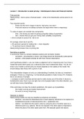
u = satisfaction of consumption. It is an increasing, concave and continuous utility function
(diminishing marginal utility: increase in happiness is increasing but at a diminishing rate):
Marginal utility = change in satisfaction. It decreases as consumption increases
There will be a maximum: a certain amount of consumption maximizes utility
At the maximum, the marginal utility is 0. One can find the maximum by finding the first
derivative of utility.
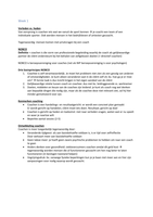
The agent’s production function is:
y1 = f(k) (1)
We use y1 to indicate that this is the amount of consumption available in the future.
k = physical capital, and also represents the agent’s savings
3
, f = an increasing, concave and continuous production function (diminishing marginal
productivity)
-> remember: for autarchy, one can only consume in the future to produce some good for
the future through the production function
The agent solves:
max u(c0, c1) = u(c0) + ꞵu(c1) (2)
What are the optimal values of c0 and c1 which maximize my utility?
Subject to:
c0 = w0 - k (3)
c1 = w1 + y1 (4)
w0 = endowment of the good which he has today e.g. paycheck/subsidy (individuals wealth)
k = savings
y1 = proceeds from production function
c0, c1 > 0 -> consumption should be non-negative
We solve this by replacing c0, c1 from the constraints into the maximand. Hence, it becomes
a one-variable problem of unconstrained optimization (as we already put the constraints in
the optimization):
max u(k) = u(w0 - k) + ꞵu(w1 + f(k)) (5)
As u is strictly concave, the first-order condition is sufficient to solve the maximization
problem:
𝑑𝑢(𝑘)
=0 (6)
𝑑𝑘
-> taking the 1st derivative of u with respect to k
We exploit the chain rule:
𝑑𝑢(𝑘) 𝑑𝑢(𝑘) 𝑑𝑐0 𝑑𝑢(𝑘) 𝑑𝑐1
= * + * (7)
𝑑𝑘 𝑑𝑐0 𝑑𝑘 𝑑𝑐1 𝑑𝑘
Intuition: k does not influence utility directly, but it does indirectly because investment affects
consumption, and in turn consumption affects utility.
Marginal utility = the increase in utility derived from one unit extra consumption. It is the
𝑑𝑢(𝑘)
derivative of utility with respect to consumption ( )
𝑑𝑐0
Hence, we obtain:
𝑑𝑢(𝑘) 𝑑𝑢(𝑘) 𝑑𝑢(𝑘)
= * -1 + * f’(k) = 0 (9)
𝑑𝑘 𝑑𝑐0 𝑑𝑐1
𝑑𝑐0
= -1
𝑑𝑘
𝑑𝑐1
= f’(k)
𝑑𝑘
Or in terms of marginal utility:
𝑑𝑢(𝑘)
= MU0 * -1 + MU1 * f’(k) = 0 (10)
𝑑𝑘
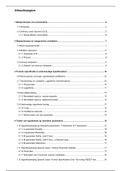
Interpretation of equation 10:
4
Time and risk
Asset pricing = how to price a financial asset -> what is the theoretically correct price for an
asset?
Two important points:
- Prices are the mirror image of returns: high price, low return
- Price and value do not always coincide (not equal when there is mispricing)
To value an asset, we consider two components:
- time = the money you want for giving up liquidity (delay of payments)
- risk = chance that you get your money back (volatility of payments)
-> time is simple to account for, risk is not
On average, stock return are 9%:
-> 8% premium earned for holding risk -> more impactful
-> 1% premium due to interest rates
Asset pricing focuses more on pricing risk
Normative vs positive
In economics, there is a tension between positive and normative models:
- normative = we prescribe a choice, how things should be theoretically (prescriptive)
- positive = what people actually do with their choices (descriptive)
Joint hypothesis problem = you can make a judgement call on mispricing only if you have a
model that works which gives you a reference point (true fundamental value). You do not
know if your model is correct and your choice depends on the validity of the model. We
should always take theory with a grinch of salt.
This interpretation shapes not only our understanding of markets, but also our investment
strategies. If there is a mispricing, it is theoretically possible to make money off it. However,
this is not obvious. Example:
-> company is worth more/less and we want to make money out of this when it returns to
fundamental value. Even if you are right, but a lot of people trade in the other direction, you
can still lose money (GameStop).
If the world does not obey the model’s predictions, this opens up 2 possibilities.
- the model is wrong and needs improvement
- the world is wrong (mispricing)
Absolute vs relative
Asset pricing models can also be classified as absolute and relative:
- absolute = we price the theoretical price of each asset by reference to its exposure to
fundamental sources of macroeconomic risk (= systematic risk)
- relative = we determine the asset’s value by using the price of another asset as a
reference point (e.g. options). We do not evaluate if the other asset is mispriced or
where the price of the other asset came from. We basically ignore risk factors.
1
,We will work with absolute consumption-based models, where:
- the trade off between current and future consumption determines investments
- investments matter to the degree that they allow investors to smooth consumption
(constant consumption over time)
The absolute approach has its limits. The CAPM for instance is a bit of a hybrid:
- the market portfolio is the main determinant of asset returns
- the return (and especially variance) on the market portfolio, or the asset betas, are
free parameters
Key equations
Asset pricing can be summed up in two equations:
- pt = E(mt+1 * xt+1)
- mt+1 = f(data, parameters)
Where pt = price (discounted expected future payoffs), xt+1 = payoff, mt+1 = stochastic
discount factor (how patient you are)
The major advantages of the discount factor approach are its simplicity and universality.
Historical perspective: we discovered
1. portfolio theory
2. mean-variance frontiers
3. CAPM (Capital Asset Pricing Model)
4. ICAPM (intertemporal)
5. APT (Arbitrage Pricing Theory)
6. option pricing
7. consumption-based model
The main hurdles in asset pricing are conceptual (meaning of what we are doing, the mind
sets) rather than mathematical.
Why do financial markets exist?
Three markets:
- Autarchy = can produce goods, but cannot trade goods (no capital market)
- Pure exchange = can trade goods, but cannot produce goods
- Exchange with production = can both trade and produce goods
There are three main assumptions:
- certainty
- = every agent perfectly knows what the consequences of their choices is ->
no risk
- one good
- = we will use wheat as numeraire, as it can be consumed and invested in
- two periods
- = there is only today and tomorrow, and investors choose how much to
consume in each period
2
,Autarchy
There are no financial markets so agents cannot trade. However, they can produce goods.
In this economy, consumption (and savings) choices are determined simultaneously with
investment choices. Intuition: agents can only save by investing in their own production
function e.g. their own firm
The agent’s utility function of the representative (= every equant is equal, they are replicas)
agent is:
u(c0, c1) = u(c0) + ꞵu(c1)
ꞵ = (1 - ẟ)-1,
with ꞵ being the subjective discount factor (which measures patience) and ẟ being the discount
rate. All agents want to consume today, so we need to discount the consumption of tomorrow.
c0 = consumption now
c1 = consumption next period
u = satisfaction of consumption. It is an increasing, concave and continuous utility function
(diminishing marginal utility: increase in happiness is increasing but at a diminishing rate):
Marginal utility = change in satisfaction. It decreases as consumption increases
There will be a maximum: a certain amount of consumption maximizes utility
At the maximum, the marginal utility is 0. One can find the maximum by finding the first
derivative of utility.
The agent’s production function is:
y1 = f(k) (1)
We use y1 to indicate that this is the amount of consumption available in the future.
k = physical capital, and also represents the agent’s savings
3
, f = an increasing, concave and continuous production function (diminishing marginal
productivity)
-> remember: for autarchy, one can only consume in the future to produce some good for
the future through the production function
The agent solves:
max u(c0, c1) = u(c0) + ꞵu(c1) (2)
What are the optimal values of c0 and c1 which maximize my utility?
Subject to:
c0 = w0 - k (3)
c1 = w1 + y1 (4)
w0 = endowment of the good which he has today e.g. paycheck/subsidy (individuals wealth)
k = savings
y1 = proceeds from production function
c0, c1 > 0 -> consumption should be non-negative
We solve this by replacing c0, c1 from the constraints into the maximand. Hence, it becomes
a one-variable problem of unconstrained optimization (as we already put the constraints in
the optimization):
max u(k) = u(w0 - k) + ꞵu(w1 + f(k)) (5)
As u is strictly concave, the first-order condition is sufficient to solve the maximization
problem:
𝑑𝑢(𝑘)
=0 (6)
𝑑𝑘
-> taking the 1st derivative of u with respect to k
We exploit the chain rule:
𝑑𝑢(𝑘) 𝑑𝑢(𝑘) 𝑑𝑐0 𝑑𝑢(𝑘) 𝑑𝑐1
= * + * (7)
𝑑𝑘 𝑑𝑐0 𝑑𝑘 𝑑𝑐1 𝑑𝑘
Intuition: k does not influence utility directly, but it does indirectly because investment affects
consumption, and in turn consumption affects utility.
Marginal utility = the increase in utility derived from one unit extra consumption. It is the
𝑑𝑢(𝑘)
derivative of utility with respect to consumption ( )
𝑑𝑐0
Hence, we obtain:
𝑑𝑢(𝑘) 𝑑𝑢(𝑘) 𝑑𝑢(𝑘)
= * -1 + * f’(k) = 0 (9)
𝑑𝑘 𝑑𝑐0 𝑑𝑐1
𝑑𝑐0
= -1
𝑑𝑘
𝑑𝑐1
= f’(k)
𝑑𝑘
Or in terms of marginal utility:
𝑑𝑢(𝑘)
= MU0 * -1 + MU1 * f’(k) = 0 (10)
𝑑𝑘
Interpretation of equation 10:
4