Statistics and Mathematics
Lec. 1: Variables, Measurement levels, Distributions
• Manifest variables: -give observable/ factual information
-only one question needed to get this information
-examples: age, gender, education leverl, holiday destination,…
• Latent variables: -give non-observable information (opposite of Manifest variables)
-many questions needed to get this information
-examples: attitudes, satisfaction, beliefs and characteristics
• Content validity: Do different items cover all oft he contents of the construct to be
measured?
• Construct validity: Does measurement scale reflect theoretical position regarding a
construct?
• Measurement levels:
Nominal scale Categorical variable
Ordinal scale = can be devided into existing categories
Interval scale Continous variable
Ration scale = “real numbers“
• Measures of central tendency: Mean = average → hypothetical value (you cannot have
└> middle point of distribution 2,6 friends)
Median = 0, 1, 1, 3, ④, 4, 4, 5, 5
Mode = most frequently mode 0, 1, 1, 3, 4, 4, 4, 5, 5
Lec. 2: Distributions and how to describe them
• Dispersion = how values differ from the mean → variation/ variance between values
• Proportion (p): e.g. total 25
6
Males 6 𝑝= 25
Female 19
6
• Variance ration (VR): e.g. 𝑉𝑅 = 1 − (25) VR = 1-p
VR = 0 → no variance in data VR = 1 → variance in data
• Interquartile range:
𝑆𝑆 ∑𝑛
𝑖=1(𝑥𝑖 −𝑥̅ )²
• Mean squared error (MS): 𝑀𝑆 = 𝑑𝑓
= 𝑁−1
(𝑥𝑖 −𝑥̅ )²
• Standard deviation (SD or s(x) or sₓ): 𝑆𝐷 = √∑𝑛𝑖=1 𝑁−1
Represents: -“fit“ of mean to data
-error
-variability in the data
,•
Nominal Mode Variance ratio Bar chart
Ordinal Mode Variance ratio Pie chart
Mean Interquartile range
Interval/Ratio Mode Variance ratio Line diagram
→ scale in SPSS Mean Interquartile range Boxplot
Median Standard deviation Histogram
• Deviations from normality
o
o Pos. kurtosis = leptokurtic
Neg. kurtosis = platykurtic
o
➢ SPSS
• Compute general things of your data
→ Analyze
→ Descriptive statistics
→ Descriptives
→ Select the variable of which you want the analysis
→ Select under Options what you want to calculate
• Plot the data
→ Graphs
→ Chart builder
→ Select the way it should be plotted (Pie, Line, Bar,…) by moving your option
, into the big field
→ Define the axis by moving the variables to the right axis
• Create new variable
→ Transform
→ Compute variable
→ Give your new variable a name under “Target variable”
→ add the variables of which you want to have a new one and divide
them by the number of variables you used
(e.g. (vari1 + vari2 + vari3 + vari4 + vari5) : 5 )
• Select variables
→ Data
→ Select cases
→ Select “if condition is satisfied”
→ Klick “If”
→ Select the variable that decides whether you keep it or not in your
analysis
→ e.g. gender=1 means you keep all the data whose gender is 1…
the others are not taken into account in your analysis
(→ if you don’t what this selection anymore,
click “data” → ”select cases”→ “All cases”)
Lec. 3: The normal Distribution, the z-transform
• Normal distribution: -used to predict probabilities that given score occurs
(𝑥−𝜇)²
1 −
𝑓(𝑥, 𝜇, 𝜎) = 𝜎 𝑒 2𝜎²
√2𝜋
𝑥𝑖 −𝑥̅
• z-transform: 𝑧𝑖 = 𝑠𝑥
afterwards: Mean = 0
SD = 1
➢ SPSS
• P-P plot
→ Analyze
→ Descriptive statistics
→ P-P plots
Lec. 1: Variables, Measurement levels, Distributions
• Manifest variables: -give observable/ factual information
-only one question needed to get this information
-examples: age, gender, education leverl, holiday destination,…
• Latent variables: -give non-observable information (opposite of Manifest variables)
-many questions needed to get this information
-examples: attitudes, satisfaction, beliefs and characteristics
• Content validity: Do different items cover all oft he contents of the construct to be
measured?
• Construct validity: Does measurement scale reflect theoretical position regarding a
construct?
• Measurement levels:
Nominal scale Categorical variable
Ordinal scale = can be devided into existing categories
Interval scale Continous variable
Ration scale = “real numbers“
• Measures of central tendency: Mean = average → hypothetical value (you cannot have
└> middle point of distribution 2,6 friends)
Median = 0, 1, 1, 3, ④, 4, 4, 5, 5
Mode = most frequently mode 0, 1, 1, 3, 4, 4, 4, 5, 5
Lec. 2: Distributions and how to describe them
• Dispersion = how values differ from the mean → variation/ variance between values
• Proportion (p): e.g. total 25
6
Males 6 𝑝= 25
Female 19
6
• Variance ration (VR): e.g. 𝑉𝑅 = 1 − (25) VR = 1-p
VR = 0 → no variance in data VR = 1 → variance in data
• Interquartile range:
𝑆𝑆 ∑𝑛
𝑖=1(𝑥𝑖 −𝑥̅ )²
• Mean squared error (MS): 𝑀𝑆 = 𝑑𝑓
= 𝑁−1
(𝑥𝑖 −𝑥̅ )²
• Standard deviation (SD or s(x) or sₓ): 𝑆𝐷 = √∑𝑛𝑖=1 𝑁−1
Represents: -“fit“ of mean to data
-error
-variability in the data
,•
Nominal Mode Variance ratio Bar chart
Ordinal Mode Variance ratio Pie chart
Mean Interquartile range
Interval/Ratio Mode Variance ratio Line diagram
→ scale in SPSS Mean Interquartile range Boxplot
Median Standard deviation Histogram
• Deviations from normality
o
o Pos. kurtosis = leptokurtic
Neg. kurtosis = platykurtic
o
➢ SPSS
• Compute general things of your data
→ Analyze
→ Descriptive statistics
→ Descriptives
→ Select the variable of which you want the analysis
→ Select under Options what you want to calculate
• Plot the data
→ Graphs
→ Chart builder
→ Select the way it should be plotted (Pie, Line, Bar,…) by moving your option
, into the big field
→ Define the axis by moving the variables to the right axis
• Create new variable
→ Transform
→ Compute variable
→ Give your new variable a name under “Target variable”
→ add the variables of which you want to have a new one and divide
them by the number of variables you used
(e.g. (vari1 + vari2 + vari3 + vari4 + vari5) : 5 )
• Select variables
→ Data
→ Select cases
→ Select “if condition is satisfied”
→ Klick “If”
→ Select the variable that decides whether you keep it or not in your
analysis
→ e.g. gender=1 means you keep all the data whose gender is 1…
the others are not taken into account in your analysis
(→ if you don’t what this selection anymore,
click “data” → ”select cases”→ “All cases”)
Lec. 3: The normal Distribution, the z-transform
• Normal distribution: -used to predict probabilities that given score occurs
(𝑥−𝜇)²
1 −
𝑓(𝑥, 𝜇, 𝜎) = 𝜎 𝑒 2𝜎²
√2𝜋
𝑥𝑖 −𝑥̅
• z-transform: 𝑧𝑖 = 𝑠𝑥
afterwards: Mean = 0
SD = 1
➢ SPSS
• P-P plot
→ Analyze
→ Descriptive statistics
→ P-P plots