Statistics = techniques for processing (large amounts of) data in different situations.
→ FEX. climate data (climate research) through the KNMI → experimental data
(treatment-control groups) → survey data etc.
→ less commonly used in qualitative research (open interviews result in data that is less
structured and less quantitative) → in this course, focus on quantitative.
→ statistical toolkit: different ways to measure, types of data, types of questions, number of
groups (1 or more), number of explanatory (independent) variables), etc.
→ what need to learn: for each situation need to decide what tool is most appropriate? how to
use it? how to interpret the results? how to draw your conclusions?
EXAMPLE: measuring differences in wind → question: are winds stronger at the coast compared
to the interior? → problem: how to measure? → at what weight, using what instrument, using
what scale → problem: how to deal with variability of data? → many places, moments (days,
moments, seasons) and times of the day → want to limit ourselves.
- Limitations of measurements: at the coast we focus on Den Helder, at the interior we
focus on De Bilt → focus on 1980-2000 → measurements at every hour in both places →
number of measurements: 2 x 20 x 365 x 24 = 350.400 scores of observations (the data).
- By means of a sample you can try to detect differences and similarities between the coast
(Den Helder) and the interior (De Bilt) → this will give an answer, but not a general
answer to the question → 2 different statistitical techniques:
- (1) Descriptive statistics: describe/summarize the data concerning the 2 groups in
tables, graphs or metrics → draw conclusions regarding similarities and differences.
- (2) Inductive statistics: can you generalize the findings for the sample to your
population? → (a) is the observed difference more than a coincidence (is the difference
statistically significant?)? → (b) what is the estimated size of the difference between the
populations?
- Measurement 1: Beaufort scale from 0-12 Bft → 0 = smoke rises straight up, 6 =
difficult to hold on to your umbrella, 9 = roof tiles are blown away, small children can
hardly stay upright → higher score indicates stronger wind → level of measurement =
ordinal (there is a certain order, but the intervals between the numbers are not
equal) → picture right shows ordinal has unequal distances.
- Measurement 2: Wind velocity in m/sec or km/h → scale from 0-infinity (in practice
to 50/200) → similar intervals on scale indicate similar difference in wind velocity →
level of measurement = interval (from 1 to 2 is similar to from 2 to 3) → if absolute 0 is
meaningful, so a score that is p times as high, indicates a wind velocity is p times as
high → level of measurement = ratio → interval and ratio are indicated by scale → picture
right shows how interval/ratio have equal distances.
- Measurement 3: used for windsurfing → 0 = too strong to windsurf, 1 = too weak to
windsurf, 2 = good for surf novices, 3 = good for experienced surfers, 4 = what Dorian van
Rijsselberghe likes (topsporters) → order of scores is not in accordance with order in
strength of wind → level of measurement = nominal (categories
cannot be ordered, FEX. different colours/departments in firms
cannot be ordered).
- Data matrix: store the big amount of data in data matrix →
columns: characteristics of the variable → rows: cases/observations,
, scores on the variables → this is data storage (doesn’t tell you much, basis for statistical
analysis) → need to transform it to have insights.
- One way to transform is via frequency table: make different
classes of the wind velocity, for each month you indicate
what is the number of observations for the category.
- This can be plotted graphically by Bar chart
with wind strength in De Bilt with Beaufort
measurement → results: less wind in July (low scores
appear more frequently) → mistake in the graph: data
is presented discreetly by seperate bars, but wind is a
continuous phenomenon (wind is not 1/2/3).
- Solve problem by Polygons: fluent line, so keeps in mind the
continuous aspect of wind → questions: what month experiences
most wind (March, because it is placed the most right)? what month
experiences most constant winds (July, because highest frequency)?
any objections against this type of graph (Beaufort scale is ordinal, so
interval between 0 and 1 is not similar to the one between 1 and 2 →
this graph suggests that these intervals are similar = an objection)?
- Can avoid this objection by using m/sec scale → most wind in
March, then November and least in July → graph is skewed
to the right (long tail at the right site, high numbers occur
frequently).
- Vergelijking De Bilt/Den Helder → how large is the
difference? can difference be expressed in a metric (how
large is difference)? different ways to answer these
questions: (a) through cumulative distribution, (b) through
difference between centers relative to distribution.
- (1) cumulative distribution: look at frequency and
then add frequency to existing frequencies (picture: at value 1.5, we have
two numbers, these have to be added on to eachother) → when frequency
= 0, there is a horizontal line → when large frequency, means steep
increase → transformed into percentages → difference measure: max
difference(∆)= max∆cp = 35.5 (difference between 2
percentages) (at value 3.5) → max difference of 100 when
FEX. the line of De Bilt is entirely above the line of Den
Helder → ∆ > 30 is large → called cut-off values.
- (2) difference between centers relative to distribution variables: look at
averages (red and blue numbers in picture) → calculate difference
between means.
Statistical toolbox:
- Mean: visualize different scores → (arithmetic) mean = Σscores/#scores = Σ
x/n (sum of the scores/number of scores) → just having a mean will not tell the
whole story → 2 movies can have the same mean, but there are differences.
- Dispersion: of the individual observations from the mean → dev = x - 𝑥 (the
mean) → sum is 0, so to look at dispersion, we need other measures → can use
2
absolute deviation = |𝑑𝑒𝑣| mean squared dev = 𝑑𝑒𝑣 → latter requires adjustment.
, 2
- Variance: 𝑠 = 𝑆𝑆/𝑑𝑓 = 𝑆𝑆/(𝑛 − 1) = 12. 5/4 = 3. 125→ df = degree of freedom
(number of deviations that are “free to vary” → sum of deviations has to be 0, so we can
freely choose 4 out of 5 deviations, but 5th is fixed to make it mount up to 0 → SS = sum
of squares (=variation) → variance is measure for dispersion of
data, the average of the squared deviations from the mean →
squaring makes each term positive so that values above the
mean do not cancel values below the mean → general idea of
the spread of your data → value of 0, means there is no
2
variability → squared metric (𝑆 ).
- Standard deviation: square root of variance gives standard
deviation (s = 𝑆𝑆/(𝑛 − 1)) → can calculate this for every
variable (for every movie) → also useful for standard normal
distribution: the mean of the distribution + and - 1 standard
deviation will contain appr. 68% of all the observations.
BACK TO EXAMPLE:
- Standard deviation: difference means can be 1.113, but mean
standard deviation can be 1.180 → means effect size D = 1.113/1.180 = 0.94
→ when D>0.8, there is a strong effect → can only take mean of the
standard deviations when the data of the 2 groups is equal, when the
data is not equal, you cannot take the mean standard deviation (in case
of different group sizes).
→ why are mean, standard deviation and effect size not appropriate? → (a) beaufort scale is
ordinal, so distances between values are meaningless, (b) distributions are skewed to the right, so
outliers bias the mean scores (have large influence) → are appropriate because: both
distributions are almost normal.
→ alternatives to ordinal measures/skewed distributions: median & quartiles:
distbrution skewed to the right → high values inflate the mean → alternative
measure for indicating the center of a sample: median → alternative measure for
dispersion: inter quartile range (IQR) (one quartile is 25%) → construct a cumulative
graph = boxplot: strong statistic for representing skewness and comparing
distributions.
When do we use descriptive statistics in research (statistics of
above): for data cleaning - for data preparation (both in method section
→ maybe constructing new variables?) - to provide insight into the
dataset (in first part of results section) → example of wind research
(picture left).
Lecture 3: Explained variation
Example 1: length of a number of students → y-axis = height → x-axis = the type of group
(male/female/combined) → Can you explain the variation in scores on one variable (Y) by
differences in scores on another variable (X)? (does gender explain part of the variation?)
- Height of students differs between genders → together (combined dispersion) more
dispersion than dispersion per gender.
- What part of the variation in Y (height) is explained by X (gender)?

