SUMMARY MRM2
Week 1 – ANOVA................................................................................................................2
Week 2 – Factorial ANOVA.................................................................................................6
Week 3 – Regression..........................................................................................................8
Week 4 – Regression (advanced) & mediation..................................................................13
Week 5 – Logistic Regression............................................................................................15
Week 6 – Factor Analysis..................................................................................................17
,Week 1 – ANOVA
PV (predicted value) OV (outcome value)
The predicted value has an effect on the outcome value.
Or:
IV (independent variable: variable that explains) DV (dependent variable: variable to be
explained)
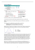
The p-value =
The probability of obtaining a result (or test-statistic value) equal to (or ‘more extreme’ than)
what was actually observed (the result you actually got), assuming that the null hypothesis is true.
A low p-value indicates that the null hypothesis is unlikely.
Conceptual models
Conceptual models = visual representations of relations between theoretical constructs (variable) of
interest (and typically also visualize the research question).
In research by “model” we mean a simplified description of reality.
Variables can have different measurement scales:
- Categorical (nominal, ordinal) – subgroups are indicated by numbers or names.
- Quantitative (discrete, interval, ratio) – we use numerical scales, with equal distances
between values.
We often use psuedo interval scales (Likert scales) = a scale from 1 till ..
Conceptual models: moderation
Conceptual models: mediation
One variable mediates the relationship between two other variables.
ANOVA = Analysis of Variance
Comparing the variability between the groups against the variability within the groups.
“How can we investigate with a certain level of (statistical) confidence, what differences there might
be between the groups?”
ANOVA is used to test whether statistically significant differences exist in scores on a quantitative
outcome variable (partner attractiveness, customer satisfaction, ...) between different levels (groups)
of a categorical predictor variable (alcohol consumption, shopping channel, ...).
The idea behind an ANOVA is to statistically investigate whether different groups score differently on
a quantitative outcome.
- How much of the variability in our outcome variable can be explained by our predictor
variable.
, - Breaks down different measurement of variability through calculating sums of squares.
- Via these calculations, ANOVA helps us to test if the mean scores of the groups are
statistically different.
We use (One way Between-subjects) ANOVA when:
- OV (outcome variable) = quantitative
- PV (predictor variable) = categorical with more than 2 groups
SSR (unexplained variance) = a part in the statistics that cannot be explained.
ANOVA steps
1. Data suited for ANOVA?
- Nature of the variables (OV = quantitative and PV = categorical)
- Assumptions met?
a) Variance is homogenous across groups. (by using the levene’s test) in PV.
b) Residuals are normally distributed (don’t test this in this class)
c) Groups are roughly equally sized (in this class they always are) (ANOVA is very sensitive
to this) in PV
d) Our subjects can only be in one group in PV
e) There are >2 groups in PV
2. Model as a whole makes sense? F-test model, R2
1. Total sum of squares (=total variance in the data)
Get the mean of all the data. Do all the (data – overall mean) 2 and add them all up.
Why square? So positive and negative numbers don’t cancel each other out.
2. Model sum of squares (=variance explained by the model)
(group mean – overall mean)2 and add them all up
Week 1 – ANOVA................................................................................................................2
Week 2 – Factorial ANOVA.................................................................................................6
Week 3 – Regression..........................................................................................................8
Week 4 – Regression (advanced) & mediation..................................................................13
Week 5 – Logistic Regression............................................................................................15
Week 6 – Factor Analysis..................................................................................................17
,Week 1 – ANOVA
PV (predicted value) OV (outcome value)
The predicted value has an effect on the outcome value.
Or:
IV (independent variable: variable that explains) DV (dependent variable: variable to be
explained)
The p-value =
The probability of obtaining a result (or test-statistic value) equal to (or ‘more extreme’ than)
what was actually observed (the result you actually got), assuming that the null hypothesis is true.
A low p-value indicates that the null hypothesis is unlikely.
Conceptual models
Conceptual models = visual representations of relations between theoretical constructs (variable) of
interest (and typically also visualize the research question).
In research by “model” we mean a simplified description of reality.
Variables can have different measurement scales:
- Categorical (nominal, ordinal) – subgroups are indicated by numbers or names.
- Quantitative (discrete, interval, ratio) – we use numerical scales, with equal distances
between values.
We often use psuedo interval scales (Likert scales) = a scale from 1 till ..
Conceptual models: moderation
Conceptual models: mediation
One variable mediates the relationship between two other variables.
ANOVA = Analysis of Variance
Comparing the variability between the groups against the variability within the groups.
“How can we investigate with a certain level of (statistical) confidence, what differences there might
be between the groups?”
ANOVA is used to test whether statistically significant differences exist in scores on a quantitative
outcome variable (partner attractiveness, customer satisfaction, ...) between different levels (groups)
of a categorical predictor variable (alcohol consumption, shopping channel, ...).
The idea behind an ANOVA is to statistically investigate whether different groups score differently on
a quantitative outcome.
- How much of the variability in our outcome variable can be explained by our predictor
variable.
, - Breaks down different measurement of variability through calculating sums of squares.
- Via these calculations, ANOVA helps us to test if the mean scores of the groups are
statistically different.
We use (One way Between-subjects) ANOVA when:
- OV (outcome variable) = quantitative
- PV (predictor variable) = categorical with more than 2 groups
SSR (unexplained variance) = a part in the statistics that cannot be explained.
ANOVA steps
1. Data suited for ANOVA?
- Nature of the variables (OV = quantitative and PV = categorical)
- Assumptions met?
a) Variance is homogenous across groups. (by using the levene’s test) in PV.
b) Residuals are normally distributed (don’t test this in this class)
c) Groups are roughly equally sized (in this class they always are) (ANOVA is very sensitive
to this) in PV
d) Our subjects can only be in one group in PV
e) There are >2 groups in PV
2. Model as a whole makes sense? F-test model, R2
1. Total sum of squares (=total variance in the data)
Get the mean of all the data. Do all the (data – overall mean) 2 and add them all up.
Why square? So positive and negative numbers don’t cancel each other out.
2. Model sum of squares (=variance explained by the model)
(group mean – overall mean)2 and add them all up