RStudio
Library() We can load the package into our R sessions
Storing a vector vector <- c(1,20,15,13,17,18,12,5)
We can also create character vectors. We use the
quotes to denote that the entries are characters
rather than variable names.
country <- c("italy", "canada", "egypt")
In R you can also use single quotes:
country <- c('italy', 'canada', 'egypt')
Sometimes it is useful to name the entries of a
vector
codes <- c(italy = 380, canada = 124, egypt = 818)
BUT class(codes)
#> [1] "numeric"
BUT with names:
names(codes)
#> [1] "italy" "canada" "egypt"
We can also assign names using the names
functions:
codes <- c(380, 124, 818)
country <- c("italy","canada","egypt")
names(codes) <- country
We use <- to assign values to the variables. We can also assign values using = instead of <-, but we recommend not
using = to avoid confusion (but if you use two == you test for equality)
Ls() is used to list the objects that are currently present in
your R session.
Rm() can be used to delete any that we don’t want. t’s also
possible to remove all objects at once: rm(list=ls())
Class() helps us determine what type of object we have
Str() is useful for finding out more about the structure of an
object
str(murders)
#> 'data.frame': 51 obs. of 5 variables:
#> $ state : chr "Alabama" "Alaska" "Arizona"
"Arkansas" ...
#> $ abb : chr "AL" "AK" "AZ" "AR" ...
#> $ region : Factor w/ 4 levels "Northeast","South",..: 2
44244122
#> 2 ...
#> $ population: num 4779736 710231 6392017
2915918 37253956 ...
#> $ total : num 135 19 232 93 1257 ...
Head() We can show the first six lines.
Or have a look at the first 50 values with:
head(na_example, n = 50)
1
,Names() We can quickly access the variable names using of the
object names(murders)
#> [1] "state" "abb" "region" "population"
"total"
Length() Tells you how many entries are in the vector. A single
number is technically a vector of length 1, but in
general we use the term vectors to refer to objects with
several entries
Levels() Factors are useful for storing categorical data. We can
see that there are only 4 regions by using the function
levels(murders$region)
#> [1] "Northeast" "South" "North Central"
"West"
$ As with data frames, you can extract the components of
a list with the accessor $. In fact, data frames are a type
of list.
record$student_id
#> [1] 1234
We can also use double square brackets ([[) like this:
record[["student_id"]]
#> [1] 1234
record2
#> [[1]]
#> [1] "John Doe"
#>
#> [[2]]
#> [1] 1234
If a list does not have names, you cannot extract the
elements with $, but you can still use the brackets
method and instead of providing the variable name, you
provide the list index, like this:
record2[[1]]
#> [1] "John Doe"
Access an element from the vector For the vector codes we defined above, we can access
the second element using:
codes[2]
Or more than 1 entry
codes[c(1,3)]
#> italy egypt
#> 380 818
if the elements have names, we can also access the
entries using these names.
codes["canada"] or
codes[c("egypt","italy")]
Matrix() We can define a matrix, we need to specify the number
of rows and columns
mat <- matrix(1:12, 4, 3)
or mat <- matrix(c(1, 2, 3, 4), 2, 2)
2
, y default R creates matrices by successively filling in
columns. Alternatively, the byrow = TRUE option can be
used to populate the matrix in order of the rows
x <- matrix(c(1,2,3,4),2,2,byrow = TRUE)
Dim() outputs the number of rows followed by the number of
columns of a given matrix
As.data.frame() We can convert matrices into data frames
as.data.frame(mat)
or
temp <- c(35, 88, 42, 84, 81, 30)
city <- c("Beijing", "Lagos", "Paris", "Rio de Janeiro",
"San Juan", "Toronto")
city_temps <- data.frame(name = city, temperature =
temp)
(You can also use single square brackets ([) to access
rows and columns of a data frame)
Seq() is used to generate sequences of numbers or other
objects. In this example, seq(1, 10) creates a sequence
of numbers from 1 to 10.
seq(1, 15, length = 5) makes a sequence of 5 numbers
that are equally spaced between 1 and 15
seq(0, 10, by = 2) makes a sequences by jumps of 2
instead of the default 1.
!! 3:11 is a shorthand for seq(3,11) !!
Table() takes a vector and returns the frequency of each
element
x <- c("a", "a", "b", "b", "b", "c")
# Here is an example of what the table function does
table(x)
#> x
#> a b c
#> 2 3 1
Sqrt() Return the square root of a number
<-> x^2 raises a number of x to the power 2
As.character() can turn numbers into characters
x <- 1:5
y <- as.character(x)
y
#> [1] "1" "2" "3" "4" "5"
As.numeric() Can you characters into numbers
As.integer() Convert vector into integers
As.factor() converts quantitative variables into qualitative variables
!! We said that vectors must be all of the same type !!
3