1.1 Microeconomics: Competitive markets - demand and supply
→ Outline the meaning of the term market
• Market: institution or mechanism that brings together buyers and sellers of good or service to carry out economic transaction
▪ Price in free market: determined solely by the interaction of supply and demand
▪ Price in controlled market: government intervenes to influence both price and output (allocation of resources)
→ Explain the negative causal relationship between price and quantity demanded.
• There is a negative causal relationship between price and quantity demanded
▪ Income effect: when price falls, people will be able to buy more as they afford more with the same amount of money
▪ Substitution effect: when price falls, the product will be more attractive than their more expensive substitutes
→ Describe the relationship between an individual consumer’s demand and market demand.
• Market demand curve: sum of all the individual demand curves in the market (represented by a demand curve)
→ Explain that a demand curve represents the relationship between the price and the quantity demanded of a product, ceteris
paribus.
• Demand: quantity of a good or service that consumers are willing and able to purchase at a given price at a given time period
▪ Demand curve: represents the relationship between the price and the quantity demanded of a product
▪ Relationship: there is a negative causal relationship between price and quantity demanded for the reasons stated above
→ Explain how factors including changes in income (in the cases of normal and inferior goods), preferences, prices of related goods
(in the cases of substitutes and complements) and demographic changes may change demand.
• Change in income
▪ Normal goods: as income rises, the demand for the product rises as people can generally afford more
▪ Inferior goods: as income rises, the demand for the product will fall as consumers purchase higher priced substitutes
▪ Taxation - changes in direct tax may affect the disposable income of individuals allowing them to afford more/less
• Price of related goods
▪ Substitutes: products that can replace one another
Relationship: increase in price of product will lead to fall in the quantity demanded for the product and
increase the demand of the substitutes which price has not changed
▪ Complements: products that are often purchased together
Relationship: increase in price of product will lead to fall in quantity demanded for the product and fall in
the demand of the complements which price has not changed
• Preferences
▪ Increased preference for a given product may increase the demand for the product, vice versa
▪ Seasonal changes: affect the needs and wants of consumers of that season (e.g. demand for ice-cream, gloves)
▪ Advertisement and marketing: preference changes as firms attempt to influence taste by advertisement and marketing
so the demand curve shifts to their favour (e.g. branding, TV advertisement of fast food)
• Demographics
▪ Change in the age structure of the population: change in the proportions of the population in different age ranges can
alter demand in favours of those groups increasing in size (e.g. aging population – reduced demand for sporting good)
▪ Change in the size of the population: if population grows, demand for most products will increase and vice versa
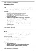
→ Distinguish between movements along the demand curve and shifts of the demand curve.
→ Draw diagrams to show the difference between movements along the demand curve and shifts of the demand curve.
• Movement along demand curve: change in ‘quantity demanded’
▪ Condition: occurs when a change in the quantity
demanded is caused only by a change in price
▪ Implies that the demand relationship (demand
curve) remains consistent and not shifted; right
• Shift of the demand curve: change in ‘demand’
▪ Condition: occurs when quantity demand is affected
by a factor other than price
▪ Implies that the original demand relationship
(demand curve) has changed (i.e. has shifted); left
→ HL content: Explain a demand function (equation) of the form Qd = a – bP.
• General equation of a linear demand curve: Qd = a – bP
▪ Qd = quantity demanded, P = price
▪ a = Q intercept, -b = slope of the demand curve
,→ HL content: Plot a demand curve from a linear function (eg. Qd = 60 – 5P).
• General demand function: Q = a – bP (e.g. Q = 60 – 5P)
• Rearranging: P = a/b – Q/b (e.g. P = 12 – Q/5)
• a/b = P intercept (e.g. 12 in Qd = 60 – 5P)
• a = Q intercept (e.g. 60 in Qd = 60 – 5P)
• -b = gradient (e.g. -5 in Qd = 60 – 5P)
→ HL content: Identify the slope of the demand curve as the slope of the demand function Qd = a – bP, that is –b
• Slope of demand function Qd = a – bP: -b is the slope
→ HL content: Outline why, if the “a” term changes, there will be a shift of the demand curve.
• Change in “a”: Q and P intercept (see above) is changed; demand curves shifts (by a constant) either way
→ HL content: Outline how a change in “b” affects the steepness of the demand curve.
• Change in “b”: P intercept and gradient (see above) is changed; steepness (ΔQ/ΔP) of the demand curve is changed
→ Explain the positive causal relationship between price and quantity supplied.
• There is a positive causal relationship between price and quantity supplied
▪ Profit incentive: at a higher price there will be more potential profits to be made and so the producers increase output
→ Describe the relationship between an individual producer’s supply and market supply.
Market supply curve: the sum of all the individual supply curves in the market.
→ Explain that a supply curve represents the relationship between the price and the quantity supplied of a product, ceteris paribus.
• Supply: quantity of good of services producers are willing and able to produce at a given price in a given time period
▪ Supply curve: represents the relationship between the price and quantity supplied of a product
▪ Relationship: there is a positive causal relationship between price and quantity demanded for the reasons stated above
→ Explain how factors including changes in costs of factors of production (land, labour, capital and entrepreneurship), technology,
and prices of related goods (joint/competitive supply), expectations, indirect taxes and subsidies and the number of firms in the
market can change supply.
• Costs of factors of production
▪ Types of factor of productions: land, labour, capital, entrepreneurship
▪ Increase in cost of a factor of production will result in producers supplying less
• Technology
▪ Improvement of technology: causes more output to be produced with same amount of input; increase in supply
▪ Cost of production: improvement of technology may also lower the cost for factor of production
• Price of related goods
▪ Competitive supply: alternative products which a firm can make with its resources
Relationship: if producers could product another product with higher profit in minimum change in
production facility, the supply for existing products decreases as producers produce more of the alternative
▪ Joint supply: product or process that can yield two or more outputs
Relationship: if there is an increase in the supply of one product, the supply of a joint product also
increases (e.g. producing more meat by cows result in more leather)
• Expectations
▪ Positive expectation: if producers expect demand to rise, the supply will increase to supply more for high profit later
▪ Negative expectation: if producers expect demand to fall, the supply will decrease to minimize profit loss later
• Government intervention
▪ Indirect tax: taxes consumer pay indirectly as part of the price of a good or service
Impact of tax: increased taxation will increase cost of production, hence forcing up the price of the product
at the same quantity supplied to maintain an adequate level of profit – decreasing their supply
▪ Subsidies: specific amount of money made by the government to firms per unit good
Impact of subsidies: increased subsidies will increase the quantity supplied of the given good or service at
the same price due to increased producer profit through government subsidy – increasing their supply
• Number of firms in the market
▪ Increased number of firms: more firms entering the market are producing the same product at each price level
▪ Decreased number of firms: less firms are producing the same product at each price level
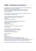
,→ Distinguish between movements along the supply curve and shifts of the supply curve.
→ Construct diagrams to show the difference between movements along the supply curve and shifts of the supply curve.
• Movement along a supply curve: change in ‘quantity supplied’
▪ Condition: refers to a change along a curve (implies
that the supply curve does not shift)
▪ Implies that the supply relationship (supply curve)
remains consistent and does not shift; right
• Shift of the supply curve: change in ‘supply’
▪ Condition: refers to a change when quantity
supplied is affected by a factor other than price
▪ Implies that the original demand relationship
(demand curve) has changed (i.e. has shifted); left
→ HL content: Explain a supply function (equation) of the form Qs = c + dP.
• General equation of a linear supply curve: Qs = c + dP
▪ Qd = quantity supplied, P = price
▪ c = Q intercept, d = slope of the demand curve
→ HL content: Plot a supply curve from a linear function (eg, Qs = –30 + 20 P).
General demand function: Q = c + dP (e.g. Qs = -30 + 20P)
• Rearranging: P = Q/d – c/d (e.g. P = 12 – Q/5)
• c/d = P intercept (e.g. -3/2 in Qs = -30 + 20P)
• c = Q intercept (e.g. -30 in Qs = -30 + 20P)
• -b = gradient (e.g. 20 in Qs = -30 + 20P)
→ HL content: Identify the slope of the supply curve as the slope of the supply function Qs = c + dP, that is d (the coefficient of P).
• Slope of supply function Qs = c + dP: -d is the slope
→ HL content: Outline why, if the “c” term changes, there will be a shift of the supply curve.
• Change in “c”: Q and P intercept (see above) is changed; supply curves shifts (by a constant) either way
→ HL content: Outline how a change in “d” affects the steepness of the supply curve.
• Change in “d”: P intercept and gradient (see above) is changed; steepness (ΔQ/ΔP) of the supply curve is changed
→ Explain, using diagrams, how demand and supply interact to produce market equilibrium.
• Equilibrium: point of agreement between producers and consumers in which the forces of demand and supply are equal
▪ Demand and supply curve interaction: equilibrium point is the intersection of the supply and the demand curve
▪ Equilibrium point: point where the quantity producers are willing and able to sell equals to the quantity consumers are
willing and able to purchase (equal force of demand and supply)
→ Analyse, using diagrams and with reference to excess demand or excess supply, how changes in the determinants of demand
and/or supply result in a new market equilibrium.
• Excess supply (surplus): when quantity supplied excessed quantity demanded at given price
▪ Shift in demand/supply curve: decrease in demand and/or increase in supply
▪ Consequence: relatively more is being supplied at the previous equilibrium price;
price has to decrease in order to reach a new equilibrium where Qd=Qs
• Excess demand (shortage): when quantity demanded excessed quantity supplied at given price
▪ Shift in demand/supply curve: increase in demand and/or decrease in supply
▪ Consequence: relatively less is being supplied equilibrium price; price has to
increase in order to reach a new equilibrium where Qd=Qs
→ HL content: Calculate the equilibrium price and equilibrium quantity from linear demand and supply functions.
• Equilibrium price: Ps = Pd a/b – Q/b = Q/d - c/d
• Equilibrium quantity: Qs = Qd dP + c = -bP + a
, → HL content: Plot demand and supply curves from linear functions, and identify the equilibrium price and equilibrium quantity.
• Equilibrium price and quantity: the respective price and quantity the demand and
supply curves intersect on a diagram
→ HL content: State the quantity of excess demand or excess supply in the above diagrams.
• Quantity of excess demand: difference in Qd and Qs when Qd > Qs at given price
• Quantity of excess supply: difference in Qs and Qd when Qs > Qd at given price
→ Explain why scarcity necessitates choices that answer the “what to produce?” question.
• Opportunity cost – there is only a limited amount of resource available hence every choice incurs an opportunity cost
• Resource allocation – resources are allocated in response to change in the market to maximize benefit to producers
→ Explain why choice results in an opportunity cost.
• Opportunity cost: opportunity cost of a choice is the value of the next best alternative given up
▪ Every choice has a possible alternative; hence every choice results in an opportunity cost
→ Explain, using diagrams, that price has a signalling function and an incentive function, which result in a reallocation of resources
when prices change as a result of a change in demand or supply conditions.
• Price mechanism: means by which consumers and producers interact to determine the allocation of scare resources
▪ Signalling function: prices adjust to demonstrate where resources are required reflecting scarcities and surpluses
Rise of price: signal to suppliers to expand production to meet higher demand
Fall of price: signal consumers to purchase more; help eliminate the surplus present in market
▪ Incentive functions: high prices will give producers an incentive to produce more of that good and vice versa
High price: provide incentive to producers to produce more of given good or service
Low price: reduce availability of suppliers to supply more of given good or service
▪ Resources are reallocated with changes in price (as a result of change in demand or supply) due to function of price
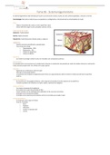
→ Explain the concept of consumer surplus.
• Consumer surplus: extra utility gained by consumers from paying a price for a given
quantity of output lower than that which is they are prepared to buy
▪ Formula: 0.5 x (Pd – Pe) x Qe = 0.5 x (AP x PB)
Pd – price where demand curve intersects the price axis
Pe/Qe – equilibrium price and quantity, respectively
→ Explain the concept of producer surplus.
• Producer surplus: excess of actual earnings that a producer makes from a given
quantity of output, above the amount the producer would be prepared to accept
▪ Formula: 0.5 x (Pe – Ps) x Qe = 0.5 x (PB x PE)
Ps – price where supply curve intersects the price axis
Pe/Qe – equilibrium price and quantity, respectively
→ Explain that the best allocation of resources from society’s point of view is at competitive market equilibrium, where social
(community) surplus (consumer surplus and producer surplus) is maximized (marginal benefit = marginal cost).
• Community surplus: total benefit to the society overall (consumer surplus and producer surplus)
▪ Competitive market: best allocation of resources in society’s point of view as community surplus is maximized
In competitive market, demand and supply determines market equilibrium price and quantity
Hence marginal benefits will equal to marginal costs, resulting in maximized community surplus
→ Outline the meaning of the term market
• Market: institution or mechanism that brings together buyers and sellers of good or service to carry out economic transaction
▪ Price in free market: determined solely by the interaction of supply and demand
▪ Price in controlled market: government intervenes to influence both price and output (allocation of resources)
→ Explain the negative causal relationship between price and quantity demanded.
• There is a negative causal relationship between price and quantity demanded
▪ Income effect: when price falls, people will be able to buy more as they afford more with the same amount of money
▪ Substitution effect: when price falls, the product will be more attractive than their more expensive substitutes
→ Describe the relationship between an individual consumer’s demand and market demand.
• Market demand curve: sum of all the individual demand curves in the market (represented by a demand curve)
→ Explain that a demand curve represents the relationship between the price and the quantity demanded of a product, ceteris
paribus.
• Demand: quantity of a good or service that consumers are willing and able to purchase at a given price at a given time period
▪ Demand curve: represents the relationship between the price and the quantity demanded of a product
▪ Relationship: there is a negative causal relationship between price and quantity demanded for the reasons stated above
→ Explain how factors including changes in income (in the cases of normal and inferior goods), preferences, prices of related goods
(in the cases of substitutes and complements) and demographic changes may change demand.
• Change in income
▪ Normal goods: as income rises, the demand for the product rises as people can generally afford more
▪ Inferior goods: as income rises, the demand for the product will fall as consumers purchase higher priced substitutes
▪ Taxation - changes in direct tax may affect the disposable income of individuals allowing them to afford more/less
• Price of related goods
▪ Substitutes: products that can replace one another
Relationship: increase in price of product will lead to fall in the quantity demanded for the product and
increase the demand of the substitutes which price has not changed
▪ Complements: products that are often purchased together
Relationship: increase in price of product will lead to fall in quantity demanded for the product and fall in
the demand of the complements which price has not changed
• Preferences
▪ Increased preference for a given product may increase the demand for the product, vice versa
▪ Seasonal changes: affect the needs and wants of consumers of that season (e.g. demand for ice-cream, gloves)
▪ Advertisement and marketing: preference changes as firms attempt to influence taste by advertisement and marketing
so the demand curve shifts to their favour (e.g. branding, TV advertisement of fast food)
• Demographics
▪ Change in the age structure of the population: change in the proportions of the population in different age ranges can
alter demand in favours of those groups increasing in size (e.g. aging population – reduced demand for sporting good)
▪ Change in the size of the population: if population grows, demand for most products will increase and vice versa
→ Distinguish between movements along the demand curve and shifts of the demand curve.
→ Draw diagrams to show the difference between movements along the demand curve and shifts of the demand curve.
• Movement along demand curve: change in ‘quantity demanded’
▪ Condition: occurs when a change in the quantity
demanded is caused only by a change in price
▪ Implies that the demand relationship (demand
curve) remains consistent and not shifted; right
• Shift of the demand curve: change in ‘demand’
▪ Condition: occurs when quantity demand is affected
by a factor other than price
▪ Implies that the original demand relationship
(demand curve) has changed (i.e. has shifted); left
→ HL content: Explain a demand function (equation) of the form Qd = a – bP.
• General equation of a linear demand curve: Qd = a – bP
▪ Qd = quantity demanded, P = price
▪ a = Q intercept, -b = slope of the demand curve
,→ HL content: Plot a demand curve from a linear function (eg. Qd = 60 – 5P).
• General demand function: Q = a – bP (e.g. Q = 60 – 5P)
• Rearranging: P = a/b – Q/b (e.g. P = 12 – Q/5)
• a/b = P intercept (e.g. 12 in Qd = 60 – 5P)
• a = Q intercept (e.g. 60 in Qd = 60 – 5P)
• -b = gradient (e.g. -5 in Qd = 60 – 5P)
→ HL content: Identify the slope of the demand curve as the slope of the demand function Qd = a – bP, that is –b
• Slope of demand function Qd = a – bP: -b is the slope
→ HL content: Outline why, if the “a” term changes, there will be a shift of the demand curve.
• Change in “a”: Q and P intercept (see above) is changed; demand curves shifts (by a constant) either way
→ HL content: Outline how a change in “b” affects the steepness of the demand curve.
• Change in “b”: P intercept and gradient (see above) is changed; steepness (ΔQ/ΔP) of the demand curve is changed
→ Explain the positive causal relationship between price and quantity supplied.
• There is a positive causal relationship between price and quantity supplied
▪ Profit incentive: at a higher price there will be more potential profits to be made and so the producers increase output
→ Describe the relationship between an individual producer’s supply and market supply.
Market supply curve: the sum of all the individual supply curves in the market.
→ Explain that a supply curve represents the relationship between the price and the quantity supplied of a product, ceteris paribus.
• Supply: quantity of good of services producers are willing and able to produce at a given price in a given time period
▪ Supply curve: represents the relationship between the price and quantity supplied of a product
▪ Relationship: there is a positive causal relationship between price and quantity demanded for the reasons stated above
→ Explain how factors including changes in costs of factors of production (land, labour, capital and entrepreneurship), technology,
and prices of related goods (joint/competitive supply), expectations, indirect taxes and subsidies and the number of firms in the
market can change supply.
• Costs of factors of production
▪ Types of factor of productions: land, labour, capital, entrepreneurship
▪ Increase in cost of a factor of production will result in producers supplying less
• Technology
▪ Improvement of technology: causes more output to be produced with same amount of input; increase in supply
▪ Cost of production: improvement of technology may also lower the cost for factor of production
• Price of related goods
▪ Competitive supply: alternative products which a firm can make with its resources
Relationship: if producers could product another product with higher profit in minimum change in
production facility, the supply for existing products decreases as producers produce more of the alternative
▪ Joint supply: product or process that can yield two or more outputs
Relationship: if there is an increase in the supply of one product, the supply of a joint product also
increases (e.g. producing more meat by cows result in more leather)
• Expectations
▪ Positive expectation: if producers expect demand to rise, the supply will increase to supply more for high profit later
▪ Negative expectation: if producers expect demand to fall, the supply will decrease to minimize profit loss later
• Government intervention
▪ Indirect tax: taxes consumer pay indirectly as part of the price of a good or service
Impact of tax: increased taxation will increase cost of production, hence forcing up the price of the product
at the same quantity supplied to maintain an adequate level of profit – decreasing their supply
▪ Subsidies: specific amount of money made by the government to firms per unit good
Impact of subsidies: increased subsidies will increase the quantity supplied of the given good or service at
the same price due to increased producer profit through government subsidy – increasing their supply
• Number of firms in the market
▪ Increased number of firms: more firms entering the market are producing the same product at each price level
▪ Decreased number of firms: less firms are producing the same product at each price level
,→ Distinguish between movements along the supply curve and shifts of the supply curve.
→ Construct diagrams to show the difference between movements along the supply curve and shifts of the supply curve.
• Movement along a supply curve: change in ‘quantity supplied’
▪ Condition: refers to a change along a curve (implies
that the supply curve does not shift)
▪ Implies that the supply relationship (supply curve)
remains consistent and does not shift; right
• Shift of the supply curve: change in ‘supply’
▪ Condition: refers to a change when quantity
supplied is affected by a factor other than price
▪ Implies that the original demand relationship
(demand curve) has changed (i.e. has shifted); left
→ HL content: Explain a supply function (equation) of the form Qs = c + dP.
• General equation of a linear supply curve: Qs = c + dP
▪ Qd = quantity supplied, P = price
▪ c = Q intercept, d = slope of the demand curve
→ HL content: Plot a supply curve from a linear function (eg, Qs = –30 + 20 P).
General demand function: Q = c + dP (e.g. Qs = -30 + 20P)
• Rearranging: P = Q/d – c/d (e.g. P = 12 – Q/5)
• c/d = P intercept (e.g. -3/2 in Qs = -30 + 20P)
• c = Q intercept (e.g. -30 in Qs = -30 + 20P)
• -b = gradient (e.g. 20 in Qs = -30 + 20P)
→ HL content: Identify the slope of the supply curve as the slope of the supply function Qs = c + dP, that is d (the coefficient of P).
• Slope of supply function Qs = c + dP: -d is the slope
→ HL content: Outline why, if the “c” term changes, there will be a shift of the supply curve.
• Change in “c”: Q and P intercept (see above) is changed; supply curves shifts (by a constant) either way
→ HL content: Outline how a change in “d” affects the steepness of the supply curve.
• Change in “d”: P intercept and gradient (see above) is changed; steepness (ΔQ/ΔP) of the supply curve is changed
→ Explain, using diagrams, how demand and supply interact to produce market equilibrium.
• Equilibrium: point of agreement between producers and consumers in which the forces of demand and supply are equal
▪ Demand and supply curve interaction: equilibrium point is the intersection of the supply and the demand curve
▪ Equilibrium point: point where the quantity producers are willing and able to sell equals to the quantity consumers are
willing and able to purchase (equal force of demand and supply)
→ Analyse, using diagrams and with reference to excess demand or excess supply, how changes in the determinants of demand
and/or supply result in a new market equilibrium.
• Excess supply (surplus): when quantity supplied excessed quantity demanded at given price
▪ Shift in demand/supply curve: decrease in demand and/or increase in supply
▪ Consequence: relatively more is being supplied at the previous equilibrium price;
price has to decrease in order to reach a new equilibrium where Qd=Qs
• Excess demand (shortage): when quantity demanded excessed quantity supplied at given price
▪ Shift in demand/supply curve: increase in demand and/or decrease in supply
▪ Consequence: relatively less is being supplied equilibrium price; price has to
increase in order to reach a new equilibrium where Qd=Qs
→ HL content: Calculate the equilibrium price and equilibrium quantity from linear demand and supply functions.
• Equilibrium price: Ps = Pd a/b – Q/b = Q/d - c/d
• Equilibrium quantity: Qs = Qd dP + c = -bP + a
, → HL content: Plot demand and supply curves from linear functions, and identify the equilibrium price and equilibrium quantity.
• Equilibrium price and quantity: the respective price and quantity the demand and
supply curves intersect on a diagram
→ HL content: State the quantity of excess demand or excess supply in the above diagrams.
• Quantity of excess demand: difference in Qd and Qs when Qd > Qs at given price
• Quantity of excess supply: difference in Qs and Qd when Qs > Qd at given price
→ Explain why scarcity necessitates choices that answer the “what to produce?” question.
• Opportunity cost – there is only a limited amount of resource available hence every choice incurs an opportunity cost
• Resource allocation – resources are allocated in response to change in the market to maximize benefit to producers
→ Explain why choice results in an opportunity cost.
• Opportunity cost: opportunity cost of a choice is the value of the next best alternative given up
▪ Every choice has a possible alternative; hence every choice results in an opportunity cost
→ Explain, using diagrams, that price has a signalling function and an incentive function, which result in a reallocation of resources
when prices change as a result of a change in demand or supply conditions.
• Price mechanism: means by which consumers and producers interact to determine the allocation of scare resources
▪ Signalling function: prices adjust to demonstrate where resources are required reflecting scarcities and surpluses
Rise of price: signal to suppliers to expand production to meet higher demand
Fall of price: signal consumers to purchase more; help eliminate the surplus present in market
▪ Incentive functions: high prices will give producers an incentive to produce more of that good and vice versa
High price: provide incentive to producers to produce more of given good or service
Low price: reduce availability of suppliers to supply more of given good or service
▪ Resources are reallocated with changes in price (as a result of change in demand or supply) due to function of price
→ Explain the concept of consumer surplus.
• Consumer surplus: extra utility gained by consumers from paying a price for a given
quantity of output lower than that which is they are prepared to buy
▪ Formula: 0.5 x (Pd – Pe) x Qe = 0.5 x (AP x PB)
Pd – price where demand curve intersects the price axis
Pe/Qe – equilibrium price and quantity, respectively
→ Explain the concept of producer surplus.
• Producer surplus: excess of actual earnings that a producer makes from a given
quantity of output, above the amount the producer would be prepared to accept
▪ Formula: 0.5 x (Pe – Ps) x Qe = 0.5 x (PB x PE)
Ps – price where supply curve intersects the price axis
Pe/Qe – equilibrium price and quantity, respectively
→ Explain that the best allocation of resources from society’s point of view is at competitive market equilibrium, where social
(community) surplus (consumer surplus and producer surplus) is maximized (marginal benefit = marginal cost).
• Community surplus: total benefit to the society overall (consumer surplus and producer surplus)
▪ Competitive market: best allocation of resources in society’s point of view as community surplus is maximized
In competitive market, demand and supply determines market equilibrium price and quantity
Hence marginal benefits will equal to marginal costs, resulting in maximized community surplus